Direct Fiber Positioning System Development |
© 2022-2023, Nathan Sayer, Open Source Instruments Inc.
© 2022, Calvin Dahlberg, Open Source Instruments Inc.
Direct Fiber Positioning System Development |
| JAN-22 | FEB-22 | MAR-22 | APR-22 | |
| MAY-22 | JUN-22 | JUL-22 | AUG-22 | |
| SEP-22 | OCT-22 | NOV-22 | DEC-22 | |
| JAN-23 | FEB-23 | MAR-23 | APR-23 | |
| MAY-23 | JUN-23 | JUL-23 | OCT-23 | |
| FEB-24 | APR-24 | MAY-24 | JUN-24 | |
| JUL-24 |
[30-MAY-24] We are building two DFPS-4A. These are based upon the DFPS-80A we proposed in our Phase II Application. The DFPS-4A is loaded with four positioners, but is built to be expanded to 80 positioners. Each positioner presents two low-NA detector fibers and one high-NA guide fiber. Our Fiducial Plate will provide four guide CCDs and four high-NA fiducial fibers. Two fiber view cameras will provide tracking of the fiducial and guide fibers. Calibration of the fiducial plate will allow us to relate the guide CCDs to the fiducial fibers. Calibration of the individual positioners will allow us to relate the detector fibers to the guide fibers. Our plan is to complete construction of the first prototype by mid-June, calibrate the first prototype by mid-August, and then ship to the McDonald Observatory in Texas for installation on their 2-m telescope. The other prototype we will have assembled and ready for diagnostic work by the time the first prototype enters service.

The DFPS-4A provides eight FC feedthroughs for optical fiber connection to a spectrograph. Four fibers are 200-μ at NA=0.12, four are 100-μ at NA=0.12. Four detector fibers and four fiducial fibers proceed to a light injector on the wall of the enclosure. Four guide sensors are arranged with the fiducial fibers on the fiducial plate around the tips of the positioner ferrules. Data acquisition takes place through a single RJ-45 ethernet socket. All power comes from a 24-V power jack. Two fiber view cameras, combined with calibration of the fiducial plate and positioner ferrules, provide the location of detector fibers with respect to the guide sensors. The high-voltage power supply is distributed to the fiber controllers, which in turn drive the electrodes of the actuators.
| Term | Meaning |
|---|---|
| Positioner | The combination of an actuator, mast, and controller that together move the tip of a fiber. |
| Actuator | The piezo-electric cylinder that bends when we apply voltage to its electrodes. |
| Mast | The long tube that acts as a lever arm to turn the bending of the actuator into translation of the fiber tip. |
| Ferrule | The cylinder with a precision center hole that presents the polished fiber tip. |
| Controller | The logic, converters, and amplifiers that generate a single actuator's four electrode voltages. |
| Base Board | The printed circuit board that supports all the positioners of a single cell. |
| Service Board | The printed circuit board that holds the fiber controllers for all the positioners of a single cell. |
| Detector Cell | A base board, its fibers, its positioners, its service board, and all its controllers. |
| Detector Fiber | A fiber used to capture and transport the light from a celestial object. |
| Guide Fiber | A fiber used to reveal the location of a detector fiber. |
| Dead Reckoning | Moving a fiber to a desired position and keeping it there with no use of guide fibers. |
| Guide Sensor | An image sensor at the edge of the positioner array that records the position of guide stars. |
| Fiducial Fiber | A fiber used to locate the positioner array with respect to celestial guide sensors. |
| Fiber View Camera | A camera looking down on the fiber tips. |
| Front End | The multi-object detector: fibers, positioners, and the fiber view camera. |
| Back End | The spectrometer itself: we plug the fibers into it and it records spectra. |
[30-MAY-24] Here are links to circuits, data sheets, drawings, and suppliers.
Drawings: Archive of solid models, model views, and fabrication drawings.Our tube actuator is a custom part made by Physik Instrumente, part number 000083725. The manufacturer describes it as "tube c255 o3,6 i2,8 L40 sCuNi". It's outer diameter is 3.6 mm, inner diameter 2.8 mm, length 40 mm.
[28-FEB-23] Our Test Stand Two (TS2) is equipped with sixteen fiber positioners. Each positioner consists of a 40-mm actuator, a 300-mm carbon-fiber mast, and 1.25-mm diameter zirconia ferrule at each end. An optical fiber runs down the center, carrying light from one ferrule to the other. In TS2, we are testing our ability to control the position of the fiber tips. We do not use the fibers to gather light from celestial objects, but instead we shine light through the ferrule at the base of each positioner and watch the movement of the fiber tip with our fiber view camera. Our focus in this Phase I development is overcoming the electrical and mechanical challenges of mounting sixteen positioners in such close proximity and controlling them individually with ±250-V actuator electrode potentials. The positioners are arrayed in a 5-mm grid, so all the electronics and mechanical fixtures must fit beneath the 20 mm × 20 mm footprint of the 4×4 array. In these efforts we have been successful.

Our Test Stand Zero (TS0) was fixed to our optical table and provided three fiber positioners. We used TS0 to study how well we can neutralize the actuator's inherent hysteresis with reset procedures, and how well we can compensate for the actuator's material creep with creep mitigation. A reset procedure consisting of a one-minute spiral movement beginning at one corner of the range of motion and ending at the center of the range provides 10 μm rms precision returning to any location in the fiber's range. Fitting a logarithmic function to the fiber position for three minutes allows us to calculate the distance it will creep with better than 10 μm rms accuracy over a half-hour period. In four months of continuous exercising of the positioners in TS0, we saw no failure of the drive electronics, no degradation of the dynamic range, nor any significant change in the creep and hysteresis of the actuators.

Our Test Stand One (TS1) was mounted in a two-axis gimbal and provided four fiber positioners. We used TS1 to continue our study of hysteresis and creep, but also to measure the deflection of the masts as we rotated the array. It was then that we discovered the steel masts sag by 700 μm when horizontal. The spreadsheet we used to calculate deflection of steel and carbon fiber masts contained two errors that together caused us to underestimate the deflection by a factor of sixty-four. We ordered custom carbon fiber masts for use in TS2. We dismantled TS1 and started working on the construction of TS2.

Test Stand Two is equipped with back-illumination for sixteen positioner and four fiducials. We can view all fibers together or we can view them separately. We aligned the positioners by hand while soldering their electrodes to the base board. The result is alignment to no better than ±0.5 mm. Our service board is missing one plug following an accident. We have fifteen plugs remaining. Of these, six are missing their 0V connection thanks to the same accident. We cannot repair the damage because we have covered the service board with epoxy to hold the remaining plugs in place. Of the nine remaining plugs, one actuator has lost all four of its connections to the base board as its electrode pin heads have broken away from the bottom layer of the base board. The remaining eight fibers move, but most do not move in a square when we drive them around there perimiter of their range of motion. Roughly one third of tour our electrode contacts are broken between the two layers of our base board.

Our TS2 control and power delivery electronics are part of a Long-Wire Data Acquisition (LWDAQ) system. A single LWDAQ root cable makes its way to our vibration-isolated optical table and connects to a LWDAQ multiplexer. All the electronics and power supplies required by TS2 are plugged into this multiplexer with LWDAQ branch cables. We read out the fiber view camera through one branch cable, control the light injector with another cable, and instruct the command transmitter with a third. Our ±250-V power supply receives ±15-V from a fourth cable. The entire system is controlled by a LWDAQ Driver with a static IP address that we can access remotely, thus permitting us to demonstrate the system while away from our laboratory.
[29-MAR-22] The Fiber Positioner Tool is available in the LWDAQ Tool menu starting with LWDAQ 10.3.6. This tool is designed to apply voltages to piezo-electric actuator cylinders in our test stands, capture images of fiber tips, plot the movement of fibers, print spot positions, and perform sequences of movements and measurements to support our study of the DFPS precision and accuracy. As our test stand expands, so will the software.

The Fiber Positioner manipulates one piezo-electric actuator and monitors one fiber tip. The program controls and reads out two Input-Output Heads (A2057H), four Slow Amplifiers (A2089E), a ±250 V Power Supply (a A2089A without potentiometers), a Contact Injector (A2080B), and a Laboratory Camera (A2075B). The contact injector provides light for the fiber. The camera is supported above the fiber and photographs its center while the fiber flashes. The Input-Output Heads provide four analog voltages that pass through the four amplifiers to produce the piezo-electric cylinder's four electrode voltages. These same Input-Output Heads provide four analog inputs to measure the electrode voltages produced by the amplifiers. Thes analog inputs are equipped with a ÷32, 30-MΩ attenuator, giving them a dynamic range of ±320 V. The Fiber Positioner provides entries for all data acquisition parameters. We have "n", "s", "e", "w" for "north", "south", "east", and "west". We have "ch" for "channel", indicating a device element number to select an output or input. The "n_out" is the eight-bit value we write to the DAC that controls the north electrode voltage, while "n_in" is the value of that voltage as measured by the "n_in_ch" analog input. Further data acquisition parameters are available in the tool's configuration panel, where we can save and un-save our configuration to disk, from which it will be loaded automatically the next time we open the Fiber Positioner tool.

Our test stand connections are shown in schematic below. Not shown are the camera connection to the LWDAQ, which monitors the fiber tip, and the contact injector that supplies light to the optical fiber running up the center of the actuator and mast. We write eight-bit control values to the DACs on the Input-Output Heads. The Input-Output Heads produce control voltages. The control voltages are amplified by the A2089Es to produce the electrode voltages.

The Move button asserts the north, south, east, and west control values, waits for the settling time, measures the electrode voltages, measures the position of the fiber image on the camera's image sensor, and reports to the data window. The fiber appears as a bright spot in the image. The spot position is the location of the centroid of this spot, measured in microns from the top-left corder of the image. The Check button measures the electrode voltages and spot position, but leaves the electrode voltages unchanged. The Zero button sets the electrode voltages to their nominal zero values, as specified by the dac_zero parameter in the configuration panel, and then performs the same actions as Move. After each step, check, or travel movement, the Fiber Positioner prints a line of numbers to its text window. The first four are the north, south, east and west control values in DAC counts, which we print in green. After that are the spot position x and y in microns from the top-left corner of the image sensor, printed in black. At the end of the line are the north, south, east, and west electrode voltages in volts.
The Travel button executes a travel script stored in a travel file. The simplest travel script consists of north, south, east, and west control values on separate lines. The Fiber Positioner sets the north, south, east, and west control values equal to these integers and executes a Move. The following example script includes comments as well as control values.
# Example Travel Script. A pound sign at the start of a line is a comment. We list
# north, south, east, and west control values separated by spaces or line breaks.
0 255 0 255
255 0 0 255
255 0 255 0
0 255 0 255
# End of list. We have driven the actuator to the four corners of its range and back again.
Each travel script line defines a travel step. The Fiber Positioner keeps track of which step it is executing with the travel index. The Step button executes the step given by the travel index and increments the travel index afterwards. The Repeat flag tells the travel to re-start from the beginning when it's done. The Trace flag tells each measurement routine to draw a line from the previous spot position to the new spot position, so we can see where the spot has been. The pass entry presents the travel script execution counter, which increments each time we execute step zero in a travel script. The loop entry presents a local counter that travel scripts can use to manage loops.
We select a travel file with Browse and modify it with Edit. We must save our modifications to disk before they will be implemented. When it executes a step, the Fiber Positioner reads the travel file, extracts the line pointed to by the travel index, prints the line to its log window, executes the line, and prints results to the data window. If the step is a comment, the Fiber Positioner takes no action other than to print the comment in the log window. In addition to comments and control values, travel steps can use the following instructions.
| Instruction | Function |
|---|---|
| label name | Label a line with alpha-numeric string name. |
| tcl s | Execute s in the TCL interpreter. |
| tcl fn | Execute file fn in the TCL interpreter. |
| wait n | Wait n seconds before proceeding to next step. |
With the tcl instruction, we execute the rest of the line as a TCL command. With tcl_source we execute a file as if it were a TCL script. We give the name of a file in the same directory as the travel script. See here for a travel script that uses tcl_source. A label instruction identifies a line so that we jump to it with the help of a TCL procedure called Fiber_Positioner_goto. The Fiber_Positioner_goto procedure takes a label name as its argument. We invoke the goto procedure within a travel script using a tcl instruction. See here for an example travel script that uses labels and jumps. The wait instruction allows us to introduce delays in our travel procedure without freezing the LWDAQ program: we can stop the wait with the Stop button, and we can continue data acquisition with other LWDAQ instruments and tools. The table below gives some example travel files.
| File | Function |
|---|---|
| Spiral.txt | Move fiber in spiral towards center of range. |
| Perimeter.txt | Move fiber around perimeter of its range. |
| Diagonal.txt | Move fiber across the diagonal of its range. |
| Hysteresis_EW.txt | Move east-west along center of range, and back. |
| Hysteresis_NS.txt | Move north-south along center of range, and back. |
| Reset_Test.txt | Start at random location, spiral reset, move to fixed location. |
| Grid_Using_Goto.txt | Spiral reset and 3×3 grid using labels and goto commands. |
| Grid_Using_Source.txt | Spiral reset and 3×3 grid using external script. |
| Creep.txt | Spiral reset, move to 3×3 grid point, monitor for 1000 s. |
The Fiber Positioner code is in the LWDAQ/Tools menu of the LWDAQ distribution. Once the Fiber Positioner is open, all its routines are available for use in travel scripts with the help of the tcl instruction. For a list of routines available to the TCL commands in travel steps, see the LWDAQ Command Reference. In Reset_Test.txt, we use standard TCL commands to generate random control values. We call Fiber_Positioner_move to assert the new control values. We write control voltages and spot position to disk with LWDAQ_print. We use the outfile variable to give us the name of the file to write to. The name in outfile is the travel file name with "_Out" appended to it. Within the TCL commands of a travel script, we have the following variables available.
| Variable | Contents |
|---|---|
| outfile | Text file for saving results, travel file name with "_Out.txt" at the end. |
| config | The Fiber Positioner's configuration array. |
| info | The Fiber Positioner's configuration array. |
| info(log) | The log window, for use with LWDAQ_print. |
| info(data) | The data window, for use with LWDAQ_print. |
| config(travel_index) | Line number of the current step, used by Fiber_Positioner_goto. |
| config(pass_counter) | Travel script execution counter, use to vary travel details. |
| config(loop_counter) | Loop execution counter, use to mange travel loops. |
| info(trace_history) | Graphical history list, set to empty string to delete. |
| info(spot_x) | Spot position, x-coordinate. |
| info(spot_y) | Spot position, y-coordinate. |
| info(n_in) | Measurement of north electrode voltage. |
| config(n_out) | Control value for north electrode. |
The pass_counter appears in the Fiber Positioner window and increments each time we execute line zero of a travel script. We can use the pass counter to change details of a travel script that we are executing multiple times. The loop_counter is also visible in the Fiber Positioner window, and we can use this counter to manage loops.
[03-JAN-22] Grant awarded.
[05-JAN-22] Finish debugging our A2089E Slow ±250-V Amplifiers. Four of them now working. Rebuild fiber positioning Test Stand, connecting digital to analog converters, amplifiers.
[03-FEB-22] Place order for 60 of 40-mm long PZ cylinders, total cost $15k. Delivery expected in 14 weeks.
[08-FEB-22] Place order for Liquid Instruments Moku:Lab electrical test instrument, a combined oscilloscope and function generator, which we plan to use to check performance of our slow, high-voltage amplifiers.
[09-FEB-22] Place order for 50 twelve-way sockets and 50 twelve-way plugs for use on 5-mm pitch PZ control circuit. Delivery expected in 12 weeks, total cost $4.4k.
[15-FEB-22] Receive Moku:Lab.
[17-FEB-22] We equip our A2057H Input-Output heads with 30-MΩ input resistors to give ÷30 monitoring of ±300 V. But the A2089E with R10 = 100kΩ cannot drive a 30 MΩ load. We drop R10 from its original 100 kΩ to 50 kΩ and we see full range ±250 V on the output while driving 30 MΩ. Voltages across R8 (316 kΩ), R9 (316 k&Omega) and R10 (50 kΩ) are 0.69 V, 0.68 V, and 0.68 V respectively. Op-amp quiescent current is 18 μA, quiescent power dissipation is 9 mW. In our stand, we view two fibers 10 mm apart at the same height as our PZ fiber and see their images separated by 1.35 mm. Our magnification is approximately 1/7.4. When we vary NS potential from −500 V to +500 V we see 3.0 mm movement of the fiber, and for EW we see 3.4 mm.
[18-FEB-22] Fiber Positioner V1.5 complete.
[24-FEB-22] We have Fiber Positioner V1.5 and use it to travel around the perimeter of our single-fiber positioner's range. Here is our travel list file. At each step, we are changing one of the control values by 64 counts.
# Fiber Positioner Travel List File
0 0 64 0 128 0 192 0
255 0 255 64 255 128 255 192
255 255 192 255 128 255 64 255
0 255 0 192 0 128 0 64 0 0
# End of File.
We cut and paste out of the Fiber Positioner text window into Results.ods and obtain the following spot position locus for fifty journeys around the perimeter.

Magnification in the image is roughly 1/7, so our 500 μm movement on the image is 3.5 mm at the fiber tip. We ramp up the control values from 0-255 and obtain the following plot of electrode voltage versus control value for the four electrodes.

When the control value is 133, the electrode voltages are in the range −5 to +5 V (average 0 V) and the control voltages are +30 to +120 mV (average 75 mV). For control values 132, electrode voltages are 5 V lower and control voltages are 80 mV lower. The dynamic range of the control voltages is ±10 V, so we expect one DAC count to be 20/256 = 80 mV. The electrode voltages saturate at ±250 V for control values 100 and 168, which produce control voltages −2.48 V and +2.76 V respectively. Our A2089E amplifiers provide gain 95 and appear to have input offset voltage 80±10 mV. We note that the A2089E circuit includes a ÷2 attenuator at the input, so the main amplifier is providing gain ×190. We drop R1 to 1.0 MΩ, R2 to 160 kΩ, and raise C3 to 100 nF. The result is ÷6, time constant 14 ms, cut-off frequency 12 Hz. The op-amp itself has 1 GΩ and 100 pF in its feedback loop, providing cut-off of 1.6 Hz, which now dominates the input network. We repeat our ramp and obtain the following.

We now use Travel_Perimeter.txt with settling_ms = 100 ms and flash_seconds 0.0003 s to trace out the perimeter of our fiber's dynamic range, and obtain the following spot position locus.

We use travel files Hysteresis_NS.txt and Hysteresis_EW.txt to obtain the following plots, where we center the cylinder in one direction and move it back and forth in the other, so as to observe the actuator's hysteresis.


Assuming magnification 1/7, we have 100 μm of hysteresis at the center of the range when returning, which is 700 μm at the fiber tip.
[28-FEB-22] We apply Reset_Test.txt to test the efficacy of a spiral reset procedure to remove hysteresis from our positioner. We begin at a random location in the ±3.5 mm dynamic range. We execute the spiral. We move to the same location half-way from the center to one corner of the range. We measure the spot position after one second and ten seconds. We repeat and tabulate below.

After ten seconds, the standard deviation of spot position is around 3 μm (1.4 and 2.6 in quadrature), which is 20 μm at the fiber tip. When we start again and repeat the experiment 75 times, we get standard deviation 5 μm, or 35 μm at the fiber tip. The long-term trend in fiber position during the two-hour experiment is roughly 5 μm.
[23-MAR-22] Release Fiber Positioner V1.7 with LWDAQ 10.3.7. Interviewed by Boston Business Journal. We have performed hundreds of travel and reset trials with the program with no errors using the setup shown below. This photograph shows our single direct fiber positioner. One 40-mm piezo-electric actuator cylinder is mounted to a platform that can support nine actuators in a 15-mm × 15-mm square. A 300-mm steel tube is glued into the end of the actuator to act as a mast. An optical fiber terminates in a 2.5-mm diameter white zirconia ferrule at the top of the mast. The optical fiber runs down the center of both actuator and mast and out through a hole in the bottom of the platform. Four ±250-V voltages enter the support platform via coaxial cables. These cause the actuator to bend, which in turn moves the tip of the fiber around in a 3.6-mm square. We shine light into the far end of the fiber and watch the tip of the fiber with a precision camera that looks down from above. The camera allows us to measure the movements of the fiber tip with 10-μm precision.
[26-MAR-22] Article published about our DFPS work in Boston Business Journal, see here.
[28-MAR-22] Release Fiber Positioner V1.8 with the addition of labels and jumps for travel scripts. New Grid_Using_Goto.txt travel script uses the pass counter to move along a 3 × 3 grid filling the dynamic range of the fiber, executing spiral algorithm at each step, with help of labels and goto statements.
[29-MAR-22] Add "tcl_source" to Fiber Positioner V1.8. New Grid_Using_Source.txt script explores 3 × 3 grid with external TCL script. We have an initial mechanical model for a fiber-packing scheme of a large detector, from which we will extract a 4 × 4 cell for our Phase I demonstration, drawing of our V1 packing is here.

Kimika writes, "The two reset procedures attempt to eliminate hysteresis, which is a tendency of a material to remember its past state. The first reset procedure is called the spiral reset procedure and it takes the following steps: A random voltage is applied for 10 seconds. The fiber is slowly spiralled to the center. A known voltage is applied and the position of the fiber is measured after 1s and 10s. We repeated steps 1-3 1230 times. We graphed the deviation of the final positions from the average and they are attached below. The standard deviation after 1s in x and y were 11.6 and 12.17, respectively. The standard deviation after 10s in x and y were 10.11 and 11.01, respectively. The second reset procedure is called the diagonal reset procedure and it takes the following steps: A random voltage is applied for 10 seconds. The fiber is driven back and forth from one extreme (500V applied) to the other extreme (-500V applied) five times. A known voltage is applied and the position of the fiber is measured after 1s and 10s. We repeated steps 1-3 1004 times. We graphed the deviation of the final positions from the average and they are attached below. The standard deviation after 1s in x and y were 14.3 and 14.3, respectively. The standard deviation after 10s in x and y were 16.4 and 18.1, respectively."

[30-MAR-22] We produce our first draft glossary of terms: actuator, mast, ferrule, base board, service board, and so on.
[31-MAR-22] If the fiber positioner is mounted upon an altitude-azimuthal mount, changes in orientation will occur only on one direction, which we could arrange to be parallel to one of axis of the fiber movement. We would then need to adjust the fiber position only along one axis during sidereal movement, which might simplify our design. We purchase a variety of carbon fiber tubes suitable for use as masts. We are looking at the deformation of the mast under its own weight as we rotate a positioner from vertical to horizontal. We re-visit our earlier calculations of mast bending, finding a significant error in our spreadsheet. Our updated table of deflections is below.

[NOTE: Due to bug in code, calculations below are a factor of 64 too low, for corrected calculation see 19OCT22.] Using the above result, we obtain the following theoretical deflections for various available tubes under their own weight. We use estimates of modulus and density from manufacturers and tables. Our calculation of the mass of 300 mm of 304H13XX is 1.34 g. We weigh one such tube and get 1.15 g.

Given that we wish to place the fiber with accuracy 10 μm rms, a maximum deflection of 10 μm or less we can tolerate without any effort at compensation. A deflection of 100 μm we would have to compensate for, but we are confident this compensation can be done with 10-μm rms accuracy. A 1-mm deflection would present us with a challenge, but we were able to predict the shape of 9-m alignment bars to within 20 μm rms while they were sagging by several millimeters in the ATLAS End-Cap Alignment System, see here.
We now consider the deflection of the mast with the weight of the ferrule at its end. Our existing ferrules are 2.5 mm zirconia with a metal flange. They weigh 0.78 g. We derive the deflection of the mast with a load at its terminus.

[NOTE: Due to bug in code, calculations below are a factor of 64 too low, for corrected calculation see 19OCT22.] We use the same formula for the area moment of inertia to obtain theoretical values for the deflection of a mast when it is horizontal with a load at the end, and tabulate below. We use 1.0 g to represent 0.78 g of ferrule and 0.22 g of fiber running down the center of the mast.

A 1.25-mm zirconia ferrule with flange has mass 0.16 g.
[01-APR-22] The Rubin Telescope optics focus light onto a 64-cm diameter area. The converging rays from the 8.4-m primary mirror subtend an angle of 44° as they meet in the focal plane. At the focal point, the approximate image blur is 0.2 arcsec, or 1 μrad. Assuming a 10-m focal length, the diameter of a distant point source is 10 μm. The pixels of the Rubin Telescope's camera are 10-μm square. If the pixel is 25 μm above or below the focal plane, the image blur increases to 20 μm. In our spectrometer, we expect to be using 100-μm diameter high-index fiber to gather light from one object. Assuming we can center the fiber on our target object with 20-μm accuracy, another 20 μm of blurring will be tolerable. The fiber tip must be within ±25 μm of the focal plane.

As our fiber moves parallel to the focal plane, in x and y, it also moves out of the plane, as shown above. Our 40-mm actuators provide θ up to 6 mrad. With mast length 300 mm, the out of plane displacement is 5.4 μm, much less than 25 μm. Even with a 400 mm mast, out of plane displacement is only 7.2 μm. Nevertheless: we must construct our fiber positioner with all fiber tips within a ±25 μm plane. Our fiber should be able to accept all rays in a ±22° cone, so its numerical aperture should be at least 0.37. The Optran Ultra WFGE fiber provides low attenuation from 400 nm to 2400 nm with numerical aperture 0.37. We can obtain this fiber with core diameter 60 μm to 220 μm.
When it comes to comparing the merits of carbon fiber and stainless steel for the mast, we note that carbon fiber, in our experience, will expand by up to 300 ppm when we take it out of 0% humidity at 20°C and place it in 100% humidity at the same temperature. With a 300-mm mast, the expansion could be as great as 100 μm, and we would fully expect 25 μm of length change during operation in a telescope dome. Meanwhile, the coefficient of thermal expansion of stainless steel is roughly 17 ppm/K. We will see a 25-μm lengthening of a 300-mm tube with a 5°C increase in temperature. So far as we can tell, the Rubin Dome interior temperature is the same as the ambient temperature at night, with efforts made to keep the temperature uniform within the dome. If we know the temperature of the fiber positioner to ±2°C, we can predict the location of the fiber tips to ±10 μm.
[08-APR-22] We have three positioners mounted on a fresh base board. The actuators are arranged on a triangle with base 14 mm and sides 10 mm. We enhance the Fiber Positioner program so it finds, plots, and records as many fibers as we enter values in the fiber elements string. We erect a new camera holder and move our test stand to our vibration-absorbing table. We note that the lens has been loose in the lens holder: we hear it rattling when we shake the camera board. We wrap teflon tape around the lens threads so the lens is secure. We adjust focus and location of camera to view all three fiber tips. Magnification in the new image is 2122 μm / 14 mm = 1/6.7. The spots range over 520-μm squares, so the fibers are moving in 3.5-mm squares.
[09-APR-22] Run a four-hour spiral-reset experiment with Grid_Using_Source.txt. We are running three positioners at once. We obtain fifteen moves to each of nine target positions. Maximum standard deviation of any fiber tip in any position is 21 μm, average is 14 μm. There is no significant trend in position versus time.
[20-APR-22] We spiral reset, move to one of the 3 × 3 grid positions, measure position, then measure again at 10 s, 20 s, and so on to 1000 s in an effort to observe the repeatability of the actuator creep. For each fiber, and each grid point with the exception of the zero point, we obtain the creep parallel and perpendicular to the movement of the fiber from the zero point, as a percentage of the length of that movement, having previously observed that the creep was roughly 3.5% per decade of time.

If we assume 5%/decade creep, the standard deviation of our error without any consultation of the actual creep will be around 3% rms. For a 2-mm movement this is 60 μm. In the perpendicular direction we see up to 6% creep. Assuming the perpendicular creep is zero will give rise to another 3% rms error of 60 μm.

Upon closer examination, we find that the creep at 100 s is always close to double the creep at 10 s, and the 1000 s is close to triple. We select six movements, two from each actuator and plot them separately.

If we assume that the creep at 1000 s will be equal to the creep from 10 s to 100 s, our error will be closer to 1% of the movement, or 20 μm for a 2-mm movement. We would accept a 100-s settling time before we could release the fibers for spectrographic use.
[25-APR-22] We have sixty hours of creep-testing. Each 1000 s is one test, in which we move all three fibers to one of the nine 3×3 grid points, including the center point that we skipped in our previous study. We have moved to 233 points, we have explored the 3×3 grid 26 times. We go through our output file and look at each coordinate of the spot position for each of the three fibers separately, so we have six sequences of numbers for each test. We skip the 1-s value and use the 10, 20, 50, 100, 200, 500, and 1000 s values. We fit a straight line to the coordinate versus the log to the base ten of the time, so this log goes from 1.0 to 3.0. We obtain the slope, intercept, and standard deviation of the residuals. We now have 1400 fits. We find that the residuals are usually of order 7 μm at the fiber tip. But there are intervals where the residual is hundreds of times higher. At times 15.2-17.2 hrs, 37.2-39.2 hrs, and 59.7-61.5 hrs we see these disturbances. Time 68.6 hrs is 1400 on Monday.
We remove the disrupted tests from our data. Of the remaining 1300 line fits, the maximum residual 13 μm rms at fiber tip and the average is only 4 μm rms. We fit a straight line to the first 500 s of measurements of each coordinate and compare the position at 1000 s to the fit. Maximum disagreement at the fiber tip is +30 μm, minimum disagreement is −30 μm, average is 0.4 μm and standard deviation is 8 μm. It appears that we can predict the coordinates of the fiber tip at time 1000 s with 8 μm precision using its path from 10-500 s. We repeat, but use only the path from 10-200 s to predict the coordinate at 1000 s. Disagreement increases to 12 μm rms.
We wrap our fiber positioner with black felt, enclosing it completely and protecting it from the air blown by our heaters and ambient light. We re-start our creep experiment at 16:00.

We would like to avoid switching between back-illumination and detection during observation. If we can place two fibers at the tip of the mast, we can use one as a guide, connecting it permanently to a light source, and use the other for detection, connecting it permanently to a spectrometer. We find dual-core stainless steel ferrule with locking pin at Thorlabs. Separation of cores is 0.7 mm. Ferrule diameter is 2.5 mm, we would rather 1.25 mm. We are looking at companies like Fiberon to see if they can make a dual-core 1.25-mm diameter ferrule.
[26-APR-22] At 14:20 we have performed 76 creep measurements since 16:00 yesterday. Each measurement takes 1058 s. For each coordinate of each of the three fibers, we predict the position at 1000 s using its variation during 10-200 s. Error in our coordinate prediction is 5 μm rms, range −28 to +36 μm. We see no period when the fibers appear to move erratically, which suggests that our Felt Tent has an effect.
We could prepare the DFPS for a one-hour exposure in the following way. We reset all fibers by spiraling them in towards the center, which takes 60 s. We move each fiber by dead reckoning to within 20 μm of its target position. We back-illuminate the fibers and measure their positions 10 s after the move. We continue monitoring the position for 190 s. We adjust the fibers to place them at the center of their target objects. We take a picture to make sure the fibers are on target. We turn off our back-illumination and begin accumulating light with all fibers. We adjust the fiber positions to compensate for creep over the next hour. At the end of the hour, the drift in fiber position due to creep will be less than 10 μm rms.
[27-APR-22] We are using the code below to parse the output file from Creep.txt. We use the value of each coordinate from 10-200 s after the move to predict the position of the fiber after 1000 s.
set fn ~/Desktop/Creep_Out.txt
set f [open $fn]
set data [split [read $f] \n]
close $f
lwdaq_config -fsd 3
set index 0
while {$index < [llength $data]-9} {
	for {set column 1} {$column <= 6} {incr column} {
		set points ""
		for {set i [expr $index+2]} {$i <= [expr $index+8]} {incr i} {
			set log_time [format %.3f [expr log10([lindex $data $i 0])]]
			append points "$log_time [lindex $data $i $column] "
		}
		LWDAQ_print $t "[lwdaq straight_line_fit [lrange $points 0 end-4]] [lindex $points end]"
	}
	set index [expr $index + 9]
}
In a spreadsheet, we subtract the actual position at 1000 s from the predicted position and plot versus time. In order to show all six coordinates provided by each creep test, we separate them along the time axis by one sixth of the creep test period. We now have forty hours of measurements with the test stand wrapped in felt. Our error is 7.4 μm rms.

[28-APR-22] This morning we note at 9:30 am the sun shining directly through a window onto the felt tent around our positioner. Without the tent, the angle of the sun is such that the tips of the fibers would be illuminated. With the felt tent, the fibers remain in the dark. We now have 63 hours of creep testing in the tent. Using 10-200 s path, our standard deviation has increased to 11 μm and we note dozens of tests in which one of the six coordinates has error greater than 50 μm. With a three-sigman cut, standard deviation drops to 9 μm. A two-sigma cut drops it to 8 μm. When we use 10-500 s standard deviation drops to 7 μm.
When it comes to routing our fibers out of a dense fiberscope, we can use connectors like these at the edges of the detector. Maximum insertion loss 0.35 dB (8%), typical 0.1 dB (2%). In the New Small Wheel upgrade of the ATLAS detector, we used optical fiber cable harnesses that joined 24 single-fiber ferrules to a single 24-fiber connector. These were made by Fibernet Ltd and cost us around $220 each.
We measure quiescent voltages in our slow amplifiers. We have dropped R10 to 50 kΩ to increase output current so that we can drive the 30-MΩ input impedance of our voltage monitor. Voltage across R10 is 0.682 V, so current is now 13.6 μA. Voltages across R8 and R9 are 0.69 V and 0.68 V respectively, for 1.7 μA through each. Total current 17 μA. We see now that R5 is insufficient, we should make it 1.0 MΩ. We propose to raise R10 to 180 kΩ to drop output current to 3.8 μA. Total current will then be 7.2 μA, quiescent power drops to 3.6 mW. We will replace R6 and R7 with a single 250 MΩ and R3 and R4 with a single 5 MΩ. To detect the output voltage, we could use the ADS7052, a 14-bit ADC in a 1.5-mm square package. Fourteen-bit precision gives us 0.3-μm resolution in a 5-mm fiber range. Suppose we monitor U1-2, where we have at 250 nA flowing through R11 when the output is at +250 V. Transistor U1 PMBTA42DS has typical current gain of 100 at 25°C and 2 μA, in which case base current is 20 nA, which is 8% of the available current. We would like to monitor ±250 V with better than 1% precision. So we will need a separate voltage divider on the actuator control voltage in order to measure it. To keep the load small and yet still read it with the ADC, we need a decoupling capacitor. We need an additional four P0805 1 GΩ resistors and six P0402 components as well as the four ADCs in order to provide monitoring. We could instead monitor the actuators by photographing their fiber tips.
[29-APR-22] We are studying the problem of mounting the positioners on a base board and plugging the controllers into the underside of the service board. Our latest drawings are here.
[02-MAY-22] We are settled upon a first draft of the mechanical design and will be submitting drawings to the machine shop this week. We will assemble positioners one at a time. A completed positioner consists of ferrule, mast, actuator, cap and second ferrule. We plug the positioners into the base board, soldering them in place as we go. The base board is counter-sunk to accept the positioner caps, and has been previously secured to a base plate with two screws. The base board is 19 mm square. It receives ±250 V sixty-four actuator control voltages through flex cables that connect the base board to the service board. These sixty-four signals constitute the Control Voltage Bus (CVB).

The service board provides sixteen connectors for sixteen controller boards. The controller boards share the same serial data bus signals and power supplies. They each produce four control voltages. The serial bus is shared with all other service boards on the same backplane, so that there could be hundreds of controllers sharing the same single-ended serial bus. The serial bus is slow: SCK will run at about 8 kHz. If a controller shorts SCK or SDI, resistors protect these signals. The SDO line is open-drain. Controllers connect it to 0V with a 1-Amp mosfet. If a controller fails with the mosfet turned on, we blow the 50-mA fuse between the controller and SDO so as to remove the controller from the bus. The backplane provides separate power supply connections for each service board. If a controller shorts a power supply, the entire service board will fail, but only this service board.

In our High-Voltage Op-Amp we have re-named resistors from the original schematic and adjusted currents for a nominal 4 mW quiescent power consumption from a 500-V power supply. The absolute maximum power supply voltage is 500 V, and both inputs must stay within 300 V of both power supply voltages.

The logic on the controller could run off a 6-μA 200-kHz clock. We divide this by 512 to get 390 Hz and use the duty cycle of this square wave to express a value between 0 and 2.5 V with 0.2% precision. We pass the 390-Hz through a low-pass filter with time constant 1.0 s, corner frequency 0.16 Hz, giving a factor of 2400 reduction in the 390-Hz component of our original square wave. This component can be at most 2.5V/2/sqrt(2) = 0.9 Vrms, so our 390-Hz ripple will be no more than 0.4 mVrms, which is 0.02% of our signal range.
[03-MAY-22] The feedback around the opamp gives a gain of ×200. An output resistor of 10 MΩ produces a time constant and voltage drop when in series with the piezo-electric tube. According to our calculations, the capacitance of our 40-mm tubes will be around 400 pF. According to the manufacturer, capacitance is of order 4 nF. We apply a 4-Vpp sinusoid through a 10-Ω resistor to the North electrode of one of our 40-mm actuators. We connect the South electrode to 0 V. We confirm that the center electrode is not connected to anything. We measure the voltages on the North electrode with a 10-MΩ probe.

The corner frequency of the low-pass response is 15 Hz, making the time constant 11 ms. The capacitance between the North and South electrodes is 11 ms ÷ 5 MΩ = 2 nF, which is consistent with each electrode having 4-nF capacitance to the central electrode. Our North-South capacitance is two 4 nF capacitors in series, or 2 nF. A 10 MΩ resistor at the output of our amplifier will introduce a time constant of 20 ms, which is negligible. Resistance of the tubes is reputed to be 1000 GΩ. We connect 10 V to the North electrode and a 10-MΩ voltmeter between the South electrode and 0 V. We see 1.5 mV on the voltmeter. We disconnect the voltmeter and see 2.6 mV. The resistance of the tube is at least 10 V ÷ 5 mV × 10 MΩ = 20 GΩ. The voltage drop across our 10 MΩ resistor will be less than 125 mV. The 10 MΩ resistor will, however, protect the power supplies from a short circuit at the fiber positioner, limiting the short circuit current to 25 μA with power dissipation 6 mW.
We have a 40-mm actuator soldered to a base board with no mast glued into it. (There previously was a mast, but while heating the tube to dry it out, the mast glue deteriorated and the mast came loose.) We connect our 10-MΩ probe to the North electrode and ground the South electrode. We flick the tube on the North side with our finger nail and see the tube generate the following voltage on its North electrode.

If the North electrode generates a negative voltage when we flick the tube to the South, we predict that a positive voltage applied to the North electrode will cause it to bend to the South.
[10-MAY-22] Our drawings for Test Stand Two are complete and in the machine shop, see Drawings.
[18-MAY-22] Received a selection of 1.25-mm diameter ferrules and sleeves. Made a hand-polished cable with 1.25 mm ferrule on one end and 2.5-mm ferrule on the other. We purchased a fusion splicing machine. Today we cleaved multimode fibers and fused them together. Work continues on schematics for the controller, service, and backplane circuits. We expect the first mechanical pieces for our sixteen-fiber prototype in three weeks.
[24-MAY-22] Met with Teresa Brainerd of BU, presented our three-fiber prototype and discussed possible collaboration with Lowell or Perkins telescopes in Arizona. The 1.8-m Perkins is owned entirely by BU and may be willing to try a new fiberscope. Unusual lens: f/17, rays at prime focus enter at ±2°, which is far smaller than the ±12° acceptance angle of a standard fiber.
We set up a photodiode and injector to measure transmission through a fiber terminated with one 2.5-mm ferrule and one ferrule or splice at the other end. We have a fiber terminated with 2.5-mm ferrules and we plug one end into an injector ten times, then the other end, and measure power out the other end, see here, our precision in measuring the 25-μW output is roughly 5%. We will be able to measure splice and connector loses of order 5%.
[25-MAY-22] Our fusion splicer appears to provide a connection between two cleaved fiber ends that loses less than 5% of the light. We start working on cleaving fibers to produce a square end that is optically flat, if this is possible. Receive 50 each of A78554 and A78557 connectors from Omnetics.
[01-JUN-22] We consider the behavior of concave mirrors. We start with the focal point of rays parallel to the mirror axis. This point moves closer to the mirror as the rays move farther from the axis.

A spherical mirror of diameter 4 m and radius of curvature 52 m will focus rays close to the axis to a point 26 m from the center of the mirror. It will focus rays 2 m from the axis to a point 19 mm closer to the mirror. The image of a star will be blurred by roughly 3 mm. All rays parallel to the axis are, however, focused perfectly to the same point if we make the mirror parabolic. The coincidence of the focal point for rays at increasing distance from the axis arises from a delightful cancelation of two second-order effects.

We now consider the focal point of rays that are not parallel to the axis. We consider three rays, one arriving at an angle α to the axis some distance above the axis, another at the same angle but the same distance below the axis, and a final ray at the same angle striking the mirror at its center. We assume the mirror provides perfect focusing for rays parallel to the axis: it is a parabolic mirror.

Here we see the fundamental limitation of the primary mirror. The focal surface is itself a parabola that bends towards the mirror. If we attempt to obtain our image with a flat image sensor, and we have objects at the center in perfect focus, objects at the edge will be blurred by the fact that they focus above the image sensor. A weakly convex lens placed immediately above the focal surface will leave the center of the field of view undisturbed, but move the focal point of peripheral rays away from the primary mirror. A suitably designed lens would flatten the focal plane. Such a lens is an example of a corrector plate. Without a corrector plate, the image of a star on a flat focal image sensor will be blurred to a diameter 2xα2, where x is the radius of the mirror. The angular blurring will be 2xα2/f. A 4-m parabolic mirror with focal length 26 m when viewing an object 2.5 mrad (9') from its axis will see the image blurred by 25 μm. In angular terms, this 25 μm is 1 μrad (0.2"). At 40' from the center, however, the blurring increases to 5".
[08-JUN-22] We get our data acquisition software running on the Raspberry Pi operating system and set up a Pi with a monitor, keyboard, and mouse to run our test stand data acquisition system over the wired Ethernet, while at the same permitting us to download results files from its drive over the wireless network. We can also log into the Pi and set up data acquisition. Our objective is to consolidate as much of our sixteen-fiber test stand onto our gimbal.

[09-JUN-22] Consider a fiberscope consisting of a primary mirror and a fiber at the image of a star. The focused rays subtend an angle θ at the fiber tip. The fiber, meanwhile, will capture all rays incident upon the polished tip of its core that are within a cone of angle β centered upon its axis. If θ > β, we lose all the light at angles greater than β, which is a fractional loss of (θ2-β2)/θ2. If θ ≤ β we capture all the light and transport it to the other end of the fiber, minus absorption loss. Light that enters the fiber core at an angle γ tends to leave the core at angle γ, as we have observed first-hand.
Although we have no photographic evidence, we make the following claim based upon many observations of optical fibers, both plastic and glas, with coherent and incoherent light, single-mode and multi-mode: after sufficient length of fiber, and with sufficient curvature of the fiber, the conical annulus will spread to become a solid cone of angle β, uniformly illuminated on our screen. No light will be lost, other than that which is absorbed by imperfections in the fiber.
The greater the angle of divergence of the light emerging from our fiber, the more challenging the design of the spectrometer optics. If light enters in a cone θ < β and emerges in a cone β, this change is irreversible: there is no optical arrangement that can restore the cone to angle θ without loss. Astronomers call this irreversible change focal ratio degradation (FRD). We can avoid FRD by matching our fiber's numerical aperture to our telescope optics. If, for example, we have light from the primary mirror in a cone θ = 11° producing 100 μm spots, we use a custom-made fiber with core diameter ≈100 μm and numerical aperture β ≈ 11°. We write to Fiberoptics Technology Inc. and hear from them that they can make optical fiber with numerical aperture as low as 0.11, for 13° cone of acceptance.
[12-JUN-22] Daniel Eisenstein points out that our earlier calculation of the focus of off-axis rays considers only the "radial" rays, not the "tangential" rays. In our original diagram, consider a family of parallel rays that reflect off the mirror at x = 0, but with varying y-coordinate dur to the curvature of the mirror. All rays encounter a surface that, in the plane of our view, is perpendicular to the mirror axis, and so reflect about the mirror axis direction.

As a result, these rays are parallel and yet separate. Their greatest separation is proportional to the square of the mirror diameter. On the focal plane, at y = f, the apparent angular spread of the light is α = s/f = (D/f)2θ/16. For diameter 4 m, focal length 20 m, the apparent angular spread of the image is 0.25% of the off-axis angle. For the same diameter, focal length 5 m, the spread is 4% of the off-axis angle.
[23-JUN-22] Mechanical parts for Test Stand Two are nearly done. We have updated the design of the base board: we will no longer screw the base board down onto the base plate. The screw holes in the base board were making the routing of tracks to the board edge impossible. We will glue the base board to the base plate. We are making a fixture to ensure correct alignment of both pieces. The base board has counter-sunk holes. We are making these by gluing two 62-mil boards together, one with 1.3-mm holes for the ferrule at the bottom of our positioner, another with 3.1-mm holes for the end plug at the bottom of the positioner. The actuators will sit on the top side of the upper circuit board.

When it comes to assembling our array of positioners, our plan is to mount all sixteen positioners on their base board, mount in a fixture, turn sideways, and solder the electrodes to their pads in a surface-mount reflow oven. We have purchased an oven for this purpose, as well as low-temperature solder paste that will reflow at 138°C, a temperature low enough that it will not damage the glue binding the actuator, mast, end plug, and base board. It is, in principle, possible to assemble the array with hand soldering, but in the long run we want to make sure all masts are vertical and we want to be able to control the height of the fibers above the base board so as to accommodate curved focal surfaces. Thus we will reflow in an oven to demonstrate a practical process for a larger instrument.
[27-JUN-22] Glass optical fibers consist of a solid, cylindrical glass core enclosed in a cylindrical glass cladding. The refractive index of the core is greater than that of the cladding, so that total internal reflection can take place at the core-cladding boundary, provided the angle of incidence of the rays propagating in the core is great enough.
When the fiber is in air, total internal reflection will occur readily at the cladding-air boundary, where the refractive index of air is far less than that of the cladding. A typical silica optical fiber has cladding of refractive index 1.458 and a core of refractive index 1.475, which is sufficient to provide numerical aperture NA = 0.22. All rays within a 22° cone centered upon the core axis will be trapped in the core by total internal reflection at the core-cladding boundary. But we note that almost all light within a 180° cone will enter the core. The only loss will be the partial reflection of light from the boundary air-glass boundary at high angles of incidence. The portion of this light that is not trapped in the core will propagate in the cladding, where it will be trapped by total internal reflection so long as the cladding is in air. With glue or plastic in contact with the cladding, the light in the cladding will escape the fiber. If the fiber is in water, with refractive index 1.33, some of this light will escape, but some will remain trapped in the cladding until the the cladding encounters glue or plastic, with refractive index greater than the cladding. Light escaping from the cladding some distance from the fiber tip gives the impression that the manner in which we are clamping or bending the fiber is causing light to escape the core. But this is not the case: the light in the core is constrained. All we are losing is the light in the cladding, which will escape eventually: sooner if we bend or touche the outer surface of the fiber.

If we match the numerical aperture of our fiber to that of our telescope optics, all the light from the primary mirror will be trapped in the core, and all the light will emerge at the other end of the fiber with the same conical angle. If we use a fiber with a numberical aperture larger than that of our telescope's rays, light will, by non-classical means, spread out in the core, so that some of it will emerge at a greater angle to the axis than it entered. Matching the fiber to the telescope is part of our plan.
We must view our fiber tips if we are to calibrate the fiber array with respect to the celestial alignment of the telescope. Daniel Eisenstein suggests that we consider placing the fiber view camera (FVC) next to the fiber array, and view the fiber array in reflection in the secondary mirror of the telescope. The secondary mirror will usually be convex, so that our view of the fiber array will be demagnified, but even if the fiber array appears to be 20 m away, our experience viewing point sources with diffraction-limited pinhole cameras suggests we can obtain 5-μrad accuracy in measuring the relative positions of fibers and fiducials, ignoring turbulence. Our calibration will be limited by turbulence, but turbulence does not increase with apparent distance, only the actual air path distance, which might be only 7 m. Mounting the FVC is now our default plan.
Our sixteen-fiber Test Stand Two will provide one fiber per positioner. But our default plan now is to place two fibers at the tip of each positioner. One fiber will run to a light injector, the other to a spectrometer. We will calibrate the relative positions of the two fibers at the positioner tip. They will be within 1 mm of one another, and we will know the vector between them with precision 10 μm, or 1%. We can illuminate each fiber individually, so our FVC does not need to provide a sharp focus that allows us to discriminate one fiber from another. A defocused image with an accurate centroid will give us greater precision.
[30-JUN-22] Nathan has been measuring actuator creep. He reports, "I converted my graphs to GIFs and put them in the temporary file. There are two graphs, the 90deg one describes the move from 1000s of 0,255 to 1000 seconds of 0,133 and measures the creep when it gets to 0,133. The 30deg one describes the same process but starts at 255,0 instead. I noted that the 30deg graph has a much greater creep in the parallel direction because it started much farther away from where we leave it. The perpendicular creep on the other hand did not exceed 5um for either movement."

The creep parallel to the movement from the reset postition is an order of magnitude larger than the creep in the perpendicular direction. If we spend 1000 s in position A, spiral reset to center position C, and move to position B, the creep is greatest in the direction BC regardless of the direction of AC.

At the end of these experiments, we break one of the three actuators on Test Stand Zero. We dismantle the test stand and prepare for Test Stand One.
[06-JUL-22] Our surface-mount re-flow oven is up and running. Our plan is to solder our actuators to their base board by mounting them in a fixture, applying solder paste to the base board, and heating them up in the oven. We can heat them to 180°C if we use 138°C melt solder paste, or 236°C if we use 183°C solder paste. We plan to glue the positioners together, so our glue must withstand the oven. We begin by studying the effect of oven temperature upon our black DP270 electronic potting epoxy.

Calvin reports, "I took M2 screws and glued them head to head with black DP270 epoxy and let them cure overnight. I then placed one into my setup as shown in the attached photo and began adding weights till the joint failed. I tested three pieces like that and recorded weights of 300g, 180g and 360g. The 180g one failed sooner I believe because I loaded it with the epoxy blob down. I also took similarly glued screws and placed them in the reflow oven on the regular cycle. The regular heating cycle I have been using for the oven begins by heating to 110°C and holding for 60 seconds. It then rapidly increases temperature to 236°C for 5 seconds before allowing the temperature to drop to 180°C for another 5 seconds and then cooling off. After this the epoxy joints became very brittle to the point that one broke in the oven and the other was easy to break with only a couple grams of pressure in my fingers. I also tried baking some epoxied screws with the low melt cycle which starts by heating to 100°C for 60 seconds, then increases to 180°C for 5 seconds, then lowers the temperature to 145°C for another 5 seconds and then cools off. This I found actually made the joints quite a bit stronger, I measured breaking weights of 700g and 650g for the two that I baked on the lower setting. I will look if there is high temperature epoxy we can buy, but it does appear that using the low melt may be an option for attachment of the masts."

[13-JUL-22] We try out J-B Weld Steel-Reinforced Epoxy (McMaster 7605A4). This glue is rated to 290°C. We glue two screws together, allow to cure overnight at room temperature and then place it in our oven. We pre-heat at 145°C for several minutes, then the oven raises the temperature to 240°C in less than a minute. The glue cracks, as shown below.


Opening up the crack, we see signs of air pockets within the glue. We mixed the glue with a stick. We will try a nozzle to reduce air bubbles and see if the glue still cracks.
[15-JUL-22] When mixed with a nozzel, the J-B Weld epoxy does not crack in our 240°C SMT reflow temperature cycle. We also test DP460 (McMaster 7467A26), a structural epoxy we have been using for decades. The DP460 turns a light shade of yellow in the 240°C cycle, but does not crumble or crack. The DP460 epoxy is rated up to 180°C. When first mixed, the J-B Weld is runny, which does not suit some of our gluing steps. But we can leave it for half an hour and it is viscous enough for our purposes. We have been gluing actuators to steel tubes with the J-B Weld, as well as ferrules to actuators and tubes, and it makes strong, reliable bonds. Another advantage of JBWeld is its cost: $8 per cartridge compared to $44 for DP460. We are willing to mix larger quantities, which results in more reliable epoxy.
We have a positioner assembly fixture. Our objective is to keep the distance from the base of the actuator to the tip of the fiber consistent to within ±100 μm, and to make the entire positioner straight to within ±0.5 mm. Later, when we assemble sixteen positioners onto a cell, we will use another fixture to arrange the fiber tips to within ±0.1 of their nominal positions. The positioner assembly fixture provides a block of plastic provides three sets of counter-sunk apertures, one set for each of three stages of assembly.
The first set is for gluing an actuator to a mast. The block is supported above a stop that holds the mast at the correct height so that the length of the actuator and mast combined will be correct. We glue four actuators to tubes. After curing, three come out of their apertures with a firm twist. One will not come out until we grab the actuator with pliers and a layer of rubber and twist. Once it starts to turn, the actuator comes free and we draw the entire mast up through the aperture. Nevertheless, we conclude that this first step is practical.
The second set of apertures is for gluing a ferrule to the mast. Each 1.25-mm diameter ferrule contains a polished optical fiber. At the other end, we must strip the 0.9-mm jacket from the fiber so that the end of the jacket is recessed several millimeters into the actuator. We glue three ferrules to three masts. When the glue is cured, we can remove one mast easil from its aperture, but the other two are well stuck. One we destroy by trying to twist it with pliers: the tube collapses. The other we are able to force out by turning the fixture upside down, placing a 1.25-mm ferrule in the aperture, and tapping the ferrule with a weight. We tap the ferrule of the collapsed tube out of its aperture also. All three ferrules now have dirt and glue on them but a little hand polishing recovers the tips of the fibers. We have no trouble hand-polishing with the mast and actuator above the ferrule. We are not sure this step is practical.
The third set of apertures is for gluing a ferrule into the base of the actuator. At the same time, we glue the protruding fiber into the ferrule. We perform this step with two ferrules. We have fiber sticking out of the tip of each. The clearance between the ferrule flange and the inner diameter of the actuator is significant. The test fixture centers them upon one another and we fill the gap with glue. Some glue is bound to seep out of the actuator and fill the plastic aperture. But we prepared one ferrule in actuator base yesterday, and to day we remove this one with a hand twist. We conclude that this step is practical.
We have a base board fixture that allows us to align the top and bottom layers of our Positioner Base Boar while we glue them with a thin layer of JBWeld. We glue the first pair of boards, using as little glue as we think will provide a bond, in the hope of avoiding any glue entering the 1.25-mm holes that will accept the ferrules.
We clean and check both our fiberscopes. One is set up for inspection of 1.25-mm ferrules, the other for 2.5-mm ferrules. We can place a positioner in the fiberscope to inspect the fiber tip any time we like, and we clean and repair the polish of the fiber tip by hand. We also have a polishing machine with custom adaptor plate set up to perform the entire polish procedure of the base ferrules.
[16-JUL-22] We have two bottom ferrules glued into actuators. They both come out of the fixture easily. Both are well-centered. One is a little crooked: the one we have to push into the actuator because the fiber jacket inside was not cut back. The other is straight and perfect. Both ferrules have fiber sticking out. We scribe, crack, and polish. Fiber looks perfect on both ends of both positioners. We have our two-layer base board prototype glued together. The joint is strong and there is no glue in any of the ferrule holes.

When we insert the base of the perfect positioner into the two-layer base board we find that the flange is longer than our counter-sink is deep, so the actuator does not sit on the surface of the base board.

The base board drawing shows the counter-sink for the flange should be 1.7 mm deep. Ours is the depth of the top board, 62 mil = 1.6 mm. The flange appears to be 0.5 mm longer than we expected. We have re-ordered the A304302X circuit board 78 mil thick, which should be perfect.
[27-JUL-22] We have our 78-mil top-layer base boards. We glue one to a bottom layer by spreading a thin layer across the top-side of the bottom layer, making sure no glue is in the holes. We clamp in our alignment fixture. The next day, there is glue in most of the holes and the holes of the bottom are off-center with respect to those of the top. We can clear the glue out of the ferrule hole by pressing a ferrule throug. But because the holes are off-center, we can't put the positioner ferrule all the way in. If we just hold the two layers together, the positioner sits perfectly. The JB-Weld glue has been 100% reliable, curing every time when mixed with a stick.

[29-JUL-22] We have 11 positioners, completed several days ago. Upon handling, we find the bond between the actuator and the mast breaks in four of the eleven. The mast and actuator are transfixed by the fiber and ferrules, but we can move the mast a few millimeters in and out of the actuator, and we can rotate the mast. We insert more glue, agitate the glue into the gap between the mast and the actuator. We lay the four positioners flat with a support for the mast to make them straight. Today they are strong and straight.
[05-AUG-22] We are considering the cost of construction of a DFPS system of various sizes: 100, 1k, 10k, and 100k fibers. As an illustration of the kind of coinstruction work required for each positioner, we refer to this time-lapse video os DESI positioner construction. We note that DESI was shut down and upgraded to overcome problems of rogue positioners bringing down the CAN bus they use to communicate with one another, see here.
[08-AUG-22] Fiber controller printed circuit boards are on their way, A3045 with solder paste stencil.
[12-AUG-22] We have our eleven perfect positioners loaded into our 16-positioner cell assembly fixture. Each positioner has on either and a MM-FER2030 ferrule with flange. The flange at the base of the actuator is unmodified and glued in place. The flange at the tip of the mast has been cut down to the same 2.4-mm outer diameter as the mast, so that it slides through the mast holder in the assembly fixture.

We have figured out how to glue the top and bottom layers of our base board together with the sixteen 1.25-mm ferrule holes centered adequately on the sixteen 3.1-mm diameter flange holes. We slide a sleeve over ten of the ferrules and find we can slide the sleeves right through the clearance holes in the base plate. Our plan is to glue the base board to the base plate.

The base plate provides a kinematic mount and a threaded hole with which we can mount the entire positioner on a support structure. In our Test Stand Two, the support structure is the bridge shown at the center of the photograph below.

One essential step in the cell assembly we have not solved: how to solder the actuator electrodes. The actuators are arranged on a 5-mm pitch grid. They are 3.6-mm in diameter. The gap between them is only 1.4 mm. If we are to hand-solder them, we must get our iron between two pairs of actuators to the inner electrodes. If we are to solder them in a reflow oven, we must apply past through the same gaps. We try hand soldering and oven reflow to get the pads on the base board welded to the electrodes on the actuator. The oven is not reliable, hand soldering is difficult. When we have sixteen independent actuators we must route sixty-four electrode voltages to the edge of the base board and this routine will be impossible on a board with 3.1-mm holes. We re-design the two-layer base board. Our new scheme involves gold-plated 9083 pins protruding from the top side of the base board to which we solder the actuators, the same pins aligning the top and bottom layers, and the heads of these pins being soldered in the reflow oven to pads on the bottom layer. Holes in the bottom layer are 1.25 mm, which makes routing sixty-four independent tracks possible. We have solder mask on all sides of both layers. We glue the bottom of the base board to the base plate with four drops of glue on the heads of the four alignment pins. Printed circuit boards are ready, we will submit for fabrication next week.
[26-AUG-22] We have firmware and software running on a hand-made Fiber Controller (A3045) circuit. Total power consumption of logic and oscillators is 1.1 mW. We have our new two-layer base board components and are assembling them together with pins.
[15-SEP-22] We make a dozen test fibers. They each have a ferrule on the end, either 1.25 mm or 2.5 mm. We connect them with sleeves. Our fusion splicer provides a light source for 2.5-mm ferrules. We use this and our adaptors from 2.5 mm to 1.5 mm to measure transmission through ferrule connections and fibers. Our results are in Fiber_Loss_1.odt. We see 5% loss for four connections, roughly 1.2% loss per connection.
[26-SEP-22] We assemble a two-layer base board with four-way connector providing access to shared electrode voltateges. We begin by soldering sixteen pins to the top layer. We push the pins through from the bottom of the board and solder them on the top side. We put solder paste on the heads of these pins. We put four alignment pins through the bottom layer of the base board. We lower the top layer down onto the bottom layer so that the four alignment pins pass through their matching holes on the top layer. When the two boards touch, the solder paste on the pin heads touches the electrode pads on the top side of the bottom layer. We solder the four alignment pins on the top side. We place in our reflow oven. All pin heads appear to be soldered to their pads. We measure resistance between electrodes and with connector footprint. All are either 0 Ω or >200 MΩ for connection and isolated respectively.

We screw a base plate into our cell assembly jig. We run four positioner ferrules into our two-layer base board. With the ferrules in their tight holes in the bottom layer of the base board, we have alignment of all components. One ferrule is reluctant to enter its aperture in the bottom layer. Its axis is not aligned well with the axis of the actuator. We have to push it harder than the others to get the ferrule to enter its aperture. We apply a drop of glue to the four alignment pin heads and press the base plate onto the base board. Now as photograph above.
We apply solder paste (183°C) to the sixteen electrode pins. We place entire jig in oven at 60°C for fifteen minutes along with excess epoxy in petry dish. Glue in petri dish is already cured. We remove petri dish and run reflow cycle on the entire jig, hoping to reflow all the electrode joints. We remove when done. Half the electrode pins are welded to their actuator electrodes. The other half have a gap between the solder on the pin and actuator. The actuator with the crooked ferrule has cracked at the base.
We remove the base plate, base board, and actuators from the jig. We complete all solder joints by hand. We weld the crack in the actuator with solder. There is a film of cured epoxy on the actuator electrodes, which makes it hard to solder to them until we have burned off the glue with our iron. We load a 4-way plug. We mount the positioner cell on our bridge.
[28-SEP-22] After soldering all electrode pins on our four-positioner cell, washing, and drying, we find that the resistance between electrodes is tens of Megaohms. We dismantle, removing the cracked actuator first. When we remove the final actuator, the resistance rises above 200 MΩ. Three of our four actuators are now broken: two cracked, one the ferrule came off the base. We observe that the inner surface of the actuators is, in fact, coated with metal, so that it forms a continuous central electrode. Our masts are not connected electrically to this electrode because of the layer of glue between the two surfaces. Some of the base ferrule flanges are connected to the center. The base flanges are near the electrodes, and their surface appears to take solder occasionally. We must be careful not to allow contact between the flanges and the electrode pins.
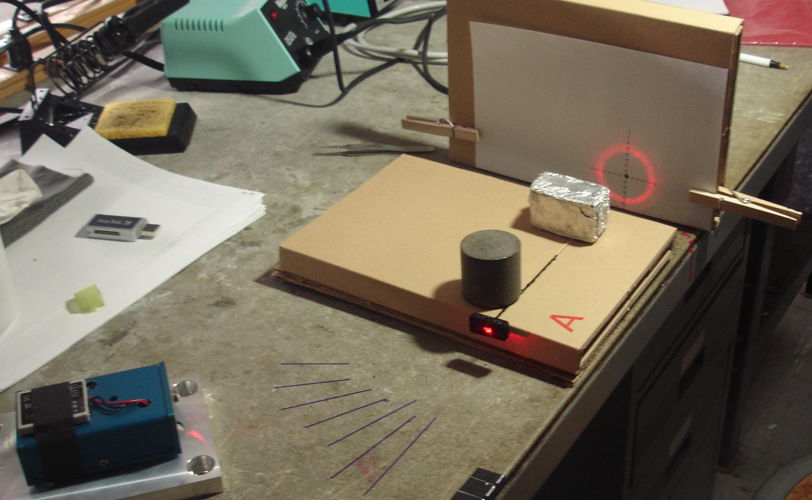
We take out three new positioners. We tin their electrodes near the base. We load into the cell assembly jig. We hand-solder all the electrode pins. We wash thoroughly, blow dry, and place in oven at 60°C for half an hour. We now see high impedance between electrodes. We load into TS1. The four 1.25-mm diameter ferrules are now accessible through apertures in the base plate. We slide sleeves onto the ferrules and connect four optical fibers. These fibers lead to a contact injector. We mount our fiber view camera and connect high voltage. See photograph.
Our fibers are not perfectly parallel: their bases are arrange on a 15 mm square but their tips are separated by up to 18 mm. Measuring the actual tip separations and comparing them to image separations, magnification in our image is 1.06 mm / 17.8 mm = 1/17. Full diagonal range of motion is 280 μm on the image sensor, for 4.8 mm at the mast tip. Our perimiter shows square of side 3.4 mm. In TS0 we were seeing squares of side 3.6 mm. In TS0 we had no ferrule glued into the bottom 5 mm of the actuator. We wonder how gluing things into the actuator might stiffen it and reduce its bending. When we apply our perimiter travel script, one of the positioners shows half the range of mostion in one direction. As we try out the new positioners, we find that changing one electrode voltage affects the others for up to one second. We see the transient electrode voltages in our Fiber Positioner Tool. The A2089E amplifier has output resistance 100 kΩ. The capacitance of the four actuators is of order 10 nF. These together would produce a time constant of only 1 ms.
[29-SEP-22] Today three fibers are moving as yesterday: two with full range, one with half-range in one direction. The fourth is barely moving. We are using our diagonal full-range travel script. We check electrode voltages on all four positioners and see ±250 V on all of them, including checking that the NS and EW potentials are always opposite ±250 V and vary independently of one another. Thus we believe there are no disconnected electrodes. And yet one actuator is no longer moving. We measure the voltage across the four 100-kΩ resistors that are in series with our electrode voltages. With the four actuators connected, we see ±800 mV across each resistor at the corners of the range of motion. While moving, however, these voltages increase to ±2 V. We disconnect the actuators and see ±780 mV accross the resistors and no increase during changes. The 7.8 μA flowing without the actuators is the current flowing into the 32-MΩ input impedance of our Input-Output Head (A2057H). The remaining 0.2 μA appears to be leaking through the four actuators. There are sixteen electrodes with 250 V across them, so we have 12 nA per electrode, so resistance of each actuator quadrant is of order 20 GΩ. During movement, we have 20 μA flowing into the actuators. We remove the weak and intert actuators and replace the two strong ones. We watch the electrode voltages and record West and South. The voltages are settling faster than they were previously.

The piezo-electric tube actuator data sheet says that the maximum "bake-out" temperature for our actuators is 150°C. We heated some of these up to 240°C in our reflow oven. The weak actuator was one that we placed in the oven. The one that failed completely we do not recall placing in the oven.
[30-SEP-22] Of the four fibers we left moving around the perimeter of their range of motion yesterday afternoon, only three are still moving correctly. A fourth, which we loaded yesterday is moving hardly at all. We apply our diagonal movement voltages and make the following recording. Using the 2.4-mm diameter masts as a reference, the movement of three of the fiber tips in the video is 4.8 mm.

[03-OCT-22] We return after three days away and find that the fiber that was unresponsive on Friday is now moving almost as far as the other three. The perimiter trace on our fiber view camera image is stable.

[04-OCT-22] The four positioners continue to move as yesterday. We rotate the stand by 45° to see how much the masts sag. We see the image positions move by 41, 41, 46, and 42 μm in the x-direction. Assuming the frame is stiff, our fiber tips are moving by 17× more, or roughly 700 μm. We receiver our A304301A rigid-flex Base and Service printed circuit boards. We load a twelve-way nano plug onto the service board, a ten-way header onto the back side. We can plug a fiber controller into the service board. We can now supply the fiber controller with power through the service board for testing.
[05-OCT-22] The four positioners are all moving together, each a distance of 250-270 μm, including the one that earlier failed to move. We are going to cut the top 150 mm off the TS1 frame so as to decrease its weight, and add a counter-weight at the bottom to balance it in the gimbal, see positioner_and_gimbal.pdf. Of four fibers we loaded into our TS1 base board, three have been moving for a week over their full diagonal range of 4.8 mm. One did not move at all on the first day after installation. The next day it was moving half as much as the other three. A week later, it is moving as much as the others. We hear from Physik Instrumente on the subject of "bake-out temperature" and the materials used in the actuators.
"Usually the CuNi-electrodes are not really suitable for this temperature range but obviously for the Reflow it seems to work. For the PIC 255 the mentioned 240°C are not critical. At least there is no complete depolarization at the temperature range but maybe a bit reduced performance but there should be any motion. The description sounds like there is a loss of contact. In case the tube itself is still ok this could happen at the edge of the soldering point but this we cannot see and check from the far. In case the customer can send us an already contacted tube please enter an RMA no. and send it to us for inspection. In this case we can check what the root cause for this could be. FYI: the critical temperature for the CuNi-electrode is usually in the range of 80-85°C. Above this level the electrode change colors and it is hard to contact the electrode. For PIC 255 we recommend a max. temperature of approx. 150°C but we know that it is quite safe up to approx. 200-220°C w/o any problems and loss in performance. Above this level it could partially Depolarize with loss in performance. Above 300°C it is very critical and depolarize significant."
We rotate the gimbal through 90° and again observe an apparant 700 μm displacement of the fiber tips. The ferrule at the end of the mast has mass 160 mg. The mast itself is 1.10 g. The fiber inside is 10 mg/cm for a total of 300 mg. Consulting our above calculations, with a 300-mm mast of 304H13XX tube, we expect displacement under its own weight of only 9 μm and with a 1-g weight only 18 μm. We calculate the bending of a PZ tube (Young's modulus is 50 GPa, density 7.8 g/cm3) with the mast attached and arrive at tens of microns. We push and pull on our high-voltage connector. The mast tips move by a couple of millemeters. While pushing on the connector, we hear a few snapping sounds. It looks like some of our solder joints from pin head to bottom layer have snapped. When we move the positioners, we hear snapping sounds. When we pull on the connector to close the gaps, the snapping stops. We turn off high voltage and wiggle the actuators. We can move them half a millimeter in any direction at the top.
[06-OCT-22] We power up the Fiber Controller (A3045) and test all four of its amplifiers as well as the four DACs and microprocessor provided by the logic. Total current consumption is 700 μA at 1V2 for roughly 1 mW, plus 45 μA at 500 V for 22 mW, total 23 mW. But there is a problem with the amplifier: it latches weakly to the negative supply rail. We can work around this issue by always driving to zero then out to our desired potential, but we will try adjusting resistors and limiting the input range to avoid saturation. We already know that increasing the output stage quiescent current from 4 μA to 14 μA provideds linear response with no latch-up, see above.
[07-OCT-22] We increase the output stage quiescent current in our high-voltage amplifiers. Their response is now linear with no latch-down. We plug two into a service board, see here. Quiescent current is 64 μA from 500 V per positioner, power consumption 32 mW. If we make a 1000-fiber spectrograph, total power dissipation will be around 32 W below the backplane, 500 mm from the focal plane. For a Stage Five Spectrograph with 50k fibers, we would dissipate 1.6 kW over a 1.2-m diameter.
[17-OCT-22] We have encased the the four actuators of this cell in epoxy at the base, so as to ensure that the actuators are mounted rigidly. We epoxy two 300-mm carbon fiber tubes next to our actuators, so that they are parallel to the steel masts when all are vertical. We now examine the tubes and the masts as we rotate the cell. When compared to the carbon fiber tubes, the masts sag by roughly 500 μm at a poing 260 mm along their 300-mm length, which is consistent with our earlier measurement of 700 μm sag in our fiber view camera, but not consistent with our calculations.
[19-OCT-22] We fasten a steel mast to a carbon fiber tube of the same length at one end, so they are parallel when vertical. When horizontal, the free tip of the steel mast is roughly 300 μm away from the carbon fiber tube. We re-examine our spreadsheet calculation and find that we forgot to convert diameter to radius and we dropped a factor of four in the moment of inertia formula. Having corrected these errors, we get the following for deflection of various tubes.

We now predict our 300-mm 304SS masts will deflect by 600 μm due to their own weight. We recalculate the effect of the weight of the ferrule, using the actual weight of the ferrule, which is 160 mg, and ignoring the distributed 300-mg weight of the fiber and its inner jacket.

The ferrule will bend our 300-mm 304SS masts by another 200 μm, making a total deflection of order 800 μm. We observed 700 μm. Our calculation assumes a mast mass of 1.34 g, but our actual masts weigh 1.1 g. We start asking carbon fiber tube manufacturers if they can make us a carbon fiber mast. We assemble our first fully-populated base board with all sixty-four electrode pins loaded. One manufacturer is looking into making us a tube OD 2.7 mm, ID 2.1 mm with carbon fiber as stiff as steel, density 1.5 g/cm3. A 300-mm mast of such tube would deflect only 200 μm.
[26-OCT-22] We have on order 20 high-modulus carbon-fiber tubes, drawing OSI-0.081HM from Clearwater Composites. Delivery is five weeks. Maximum OD of these tubes will be 0.108" at one end, or 2.74 mm, which is less than the 2.8-mm inner diameter of our actuators. Inner diameter is 0.081", or 2.06 mm, which is large enough to accommodate the flange of our 1.25-mm diameter ferrule, see here.
[17-NOV-22] We have two Fiber Controllers with fully-functional analog circuits. Firmware running in logic chip ramps up and down the electrode voltages using its four serial digital to analog converters.
[22-NOV-22] We have reserved a booth at the American Astronomical Society meeting in Seattle in January.
[12-DEC-22] New carbon fiber masts have arrived, allowing us to proceed with production of our first complete set of fiber positioners.

[15-DEC-22] The carbon fiber in the masts is M46J. According to Clearwater Composites, modulus of our tubes is 28.37 msi (megapounds per square inch) in flexure and 29.06 msi in tension, which is roughly 200 GPa. That's higher than the 140 GPa we assumed in our tables above. So we make a new table for these tubes.

Total deflection of a 300-mm mast with a 1.25-mm flanged ferrule at the end is around 200 μm. That's four times less than the deflection we expect from a steel mast.
[16-DEC-22] We begin assembly of sixteen positioners with carbon-fiber masts. Our existing fixtures have 2.4-mm holes for our former steel masts. Our new masts are 2.6-mm in diameter. Instead of waiting for our fixtures to be modified, we make impromptu fixtures to glue the positioners together. We begin by gluing four actuators to masts.
[21-DEC-22] We have eight carbon-fiber tubes glued into eight actuators. We set up for the first time serial communication with our fiber controller circuit. We connect and adapted radio-frequency Command Transmitter (A3029), which we call the A3029F. This circuit provides the serial transmission as well as the five-volt power supply required by our Backplane (A3044BP-A). We plug a Base and Service Board (A3043) into our Backplane. We plug a Fiber Controller (A3045) into the Service Board, see below.
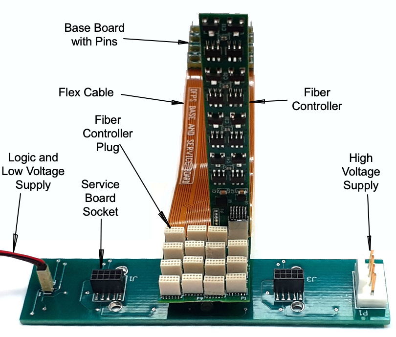
We use our existing Stimulator Tool program to send commands through the A3029F, the A30344, the A3043, and so to the A3045. We work on the A3045 firmware and release version v1.3. We can set the electrode digital to analog converters (DACs), we can start and stop a self test. The fiber controller responds only to commands addressed to its own sixteen-bit identifier, or to the wildcard identifier.
[30-DEC-22] Fiber controllers responding to individual identifier numbers while mounted in cell with sixteen connectors. Measure voltage linear from −244 V to +252 V, stable and linear. Backplane, service board, base board, fiber controller boards all working together.
[04-JAN-23] We have finalized component values in our high-voltage amplifiers, having obtained the following performance from two identical fiber positioners.
We see full range ±250 V. Non-linearity is 7 V rms from −240 to +240 V. Output votages are stable to ±0.1 V over 100 s, which is 0.02% of full range, which is of order 1 μm stability for dynamic range 3.8 mm at the mast tip. Controllers are consuming 75 μA total each with no load on the amplifiers. Total power consumption per fiber positioner is 75 μA × 500 V = 37.5 mW plus 2.5 mW from the logic power supply for the ring oscillator is 40 mW/fiber.
[09-JAN-23] We complete assembly of our first carbon-fiber positioner. The fibers are polished at both ends. Despite a film of glue residue over the actuator base, we are able to apply solder to all four electrodes. We have four completed, programmed, and tested fiber controllers, all have passed Quality Controle One (QC1). Output voltages versus input DAC values as shown below.

We receive three new cell base plates, bringing our total to five. We are opening holes in our cell assembly fixture to accommodate the carbon fiber masts.
[12-JAN-23] We have five complete fiber positioners. They are almost perfect: two of them have mast ferrules pointing a few degrees from the axis of the mast. It turns out that the skew in the tip ferrules is due to burrs on their circumference, see below.

Assembly of a single positioner takes four days. On the first day, we glue four masts into four actuators. We prepare the internal fiber and glue its mast-tip ferrule onto one end. On the second day we cleave and polish the fiber in the mast-tip ferrule. We thread the fiber down the center of the positioner, mount in our assembly fixuture so that it is vertical, and glue the mast tip ferrule into the tip of the mast. On the third day we glue the mast base ferrule onto the base end of the optical fiber. At the same time we glue the base ferrule into the base of the actuator. We place these in our assembly jig, which holds the ferrule straight and flush against the actuator base. On the fourth day we cleave the base fiber, clean epoxy residue off the base ferrule, polish the fiber in the base ferrule, and our positioner is complete. Performing all these tasks on four sets of parts takes two hours per day. Thus two hours per day suffices to produce four fiber positioners per day. In quantity 250, the masts are $50, the actuators would be around $200, ferrules and fiber around $20, labor including overhead 2 × $50 = $100. Fiber positioners in quantity 250 would cost about $370 and we could produce them four per day without much trouble, so all 250 in a few months.
[13-JAN-23] We break one actuator when removing it from our assembly fixture. Today we have three positioners with base ferrule curing, four positioners with tip ferrule curing, and four positioners with mast curing in actuator.

We use our cell assembly jig to align four fiber positioners, one after another, and solder their electrodes to the base board electrode pins. We shatter one actuator in the process, but we have one spare, so we carry on. When we load the fourth positioner, we encounter a long-anticipated problem: one of the electrode pins is obstructed by the other positioners. We use our grinding wheel to create a narrow soldering tip that can pass between the actuators to the obstructed pin.

With this bit we reflow all joints. We clean in hot water with a brush and compressed air. We mount again in the assembly fixture. We have the base ferrules clasped to the base board with sleeves. We align the base board with a base plate. With four drops of epoxy we glue the two together at the four pin heads under the base board. Visual inpsection reveals that the alignment between the base board and plate is not perfect. We adjust set screws on the stages until holes in base board appear centered on holes in base plate holder. Leave to cure.

[21-JAN-23] We have a base plate glued to our base board. We attach the base plate to a larger plate using its kinematic mount and single screw. We stand the cell upright. We tin the electrodes of nine positioners. We solder the nine positioners into place, aligning them by hand and by eye. We use our bent soldering tip to reach behind the actuators. We wash in hot water and try. With the masts vertical and no voltage applied to any actuator, the distance between mast tip fibers and their four nearest neighbors is 4-6 mm, suggesting our alignment is accurate to ±0.5 mm.

We now have all but three of sixteen positioners loaded. We expect to have another five ready to load by Monday afternoon. We have five of sixteen fiber controllers tested and running, and another thirteen near completion.
[23-JAN-23] We have four more positioners ready. We load three more onto our cell, making up the total to sixteen. The array of 4×4 is complete. We mount on our gimbal and connect all sixteen fibers to a Contact Injector (A2080). We obtain the following image of sixteen fibers shining. The entire Test Stand Two now looks like this.

[26-JAN-23] We load the backplane onto the underside of our bridge, connect logic signal and power, plug our service board into the backplane, and plug a single fiber controller into the service board. We connect ±250 V to the backplane. We hear a spark. The backplane the wrong way around. The service board plug is rotated 180°. We remove the backplane and load it the right way around. We reconned all electronics. We see ±250 V on the fiber controller, but the amplifiers are not responding to commands. We have damaged the controller.
[01-FEB-23] Our service board has fifteen of sixteen connectors loaded and fixed in place with epoxy. One connector, P12, is missing because we ripped it off. We now find that six of the remaining connectors are missing their 0V connection, we assume because of damage done to the shared 0V trace when we ripped off P12. Of the nine plugs that provide all necessary connections to the fiber controller, we see movement at the tip of our fiber positioner in all but one, the one connected to P4. We checked all connections between the pins and the connector pads before we loaded the connectors. Since them, we have stressed the bond between the top and bottom layers of the base board. The P4 positioner is on a corner, where the pin head solder joints would be subject to the greatest stress.
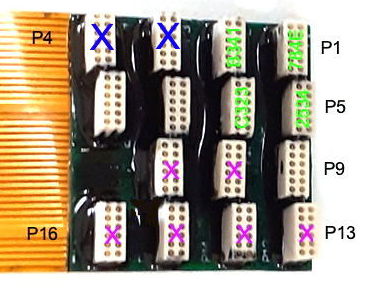
We have seven moving masts. Most are providing what looks like full range of motion along the diagonal, but a few are moving less, which suggests one or more of their electrodes pins is not in contact with its pad on the base board. The joints between the actuator electrodes and the pins are all visible and correct.
[02-FEB-23] We load our four fiducial fibers into the frame around our sixteen fiber positioners. The fiducials are arranged in a 50-mm cross (a square with sides 35-mm sides). On the image sensor, the horizontal 50 mm appears as 3283 μm, so magnification is 1/15.23. In the vertical direction, 50 mm is 3284 μm, magnification 1/15.22.
Our connected fibers are P1, P2, P5, P6 in a block of 2 × 2. They fit together nicely. We try to move them along the perimiter of their diagonal range. We see the following loci traced out in the Fiber Positioner Tool. Only one positioner moves in a 45° rotated square. Its diagonal movement is 271 μm on the image sensor, or 4.1 mm. The square has side 2.9 mm.

We adjust each electrode voltage in turn. P1 has SE, P2 has NSEW, P5 has SE, P6 has SEW. We determine also that a positive voltage on an electrode makes that quadrant of the actuator expand, so that the mast tip bends in the opposite direction to the name of the electrode. Thus we apply a positive voltage to S and the masts move north.
[07-FEB-23] We have eleven controllers fully functional and loaded onto the service board. Seven actuators move to varying degrees. We can move each actuator individually, or all actuators together.

[08-FEB-23] We have seven fiber controllers loaded on our service board: we remove those that serve no purpose. Our allocation of service boards to plugs and contact injector channels is below.

Of the seven positioners that move, three move in the correct squares. We set all seven to moving in the same perimeter pattern. By moving all seven, we avoid a couple of collisions that arise because of the poor initial arrangement of the mast tips. We flash the tips of the three good positioners and trace out their movements.

We take the measured positions of the fiber tip image on our image sensor, combine with the known magnification, and deduce that the sides of these squares are 3.1 mm. Their diagonals are 4.3 mm.

We rotate our gimbal so that our positioners are horizontal, move through vertical, and back to horizontal again in the other direction. In each orientation, we measure the position of our three good positioners and the three fiducial fibers that are well within the view of our camera. We have high voltage power turned on, and all electrode DACs set to 0x7D00, which produces electrode voltages within a few volts of zero. As we rotate the gimbal, the mast tips move by ±350 μm.

We have concluded that we should mount the actuators on the base board first. We would like to find some way to connect the actuators to the base board with pins and sockets. We try silicone-insulated stainless steel spring leads, 0.7 mm in diameter terminated with sockets. We solder these leads one third of the way up our actuators, four for each actuator. We wash and dry. On the base board, we use only the lower layer of the sandwich, and upon this lower layer we solder pins facing straight up. We wash and dry. Now we can slide the sockets onto the pins one at a time with tweezers while the actuator is to one side. We try to place the actuator on the board between the pins, but we need to change the orientation of the sockets, and the leads themselves are a little large, we might do better with our 0.5-mm leads. Hand-soldering the actuators without the masts would be easier than doing so with the masts. Either way: we believe we can mount the actuators efficiently on the base board so long as the masts are not yet loaded. With actuators secured, we can load all sixteen masts at the same time in a fixture, gluing them in place and aligning them perfectly with the fixture. Now that the full cell of actuators and masts is assembled, we can thread our fiber down from the mast tip and out the bottom. In this procedure, we have no ferrule at the base. Instead we have a ferrule that emerges from the bottom, we pull it some distance aside, and couple to another fiber far from the cell.
[10-FEB-23] We build a ±250-V isolated power supply that we supply with ±15-V from the LWDAQ. Our electronics is now as shown here. The entire Test Stand Two (TS2) is powered and controlled by a single LWDAQ root cable. Current consumption is 110 mA from ±15V (the two 250-V converters) and 50 mA from +5V (35 mA to the Command Transmitter). We have assigned the LWDAQ driver a static IP address that is visible to the outside world.
We try out an idea for eliminating solder joints on the base board: we solder silicone-insulated helical leads to the actuator, solder sockets to the end of these leads, and slide the sockets down onto pins that are surface-mounted onto the base board.

We are unable to load the actuator in the space between the sockets, because on this base board the pads for the pin heads are too close together. These leads are 0.7 mm in diameter, we also have available to us 0.5-mm diameter leads, and these will take up less space. The breakdown voltage of this one-part vulcanizing silicone is roughly 10 kV/mm, so we need at least 50 μm of silicone to insulate the lead inside from an actuator electrode 500-V away.
[16-FEB-23] Nathan Sayer (Engineer) and Kevan Hashemi (Engineer) of OSI visiting Darren DePoy (Proffessor), Jennifer Marshall (Proffessor), Luke Schmidt (Scientist), Ryan Oelkers (Scientist), Erika Cook (Engineer) of Texas Agrigulture and Mining University (TAMU) in College Station, Texas. Talks by Nathan PZ Actuators, by Kevan Introduction and Hardware, by Luke McDonald 82-Inch and Spectrometer Options.
[17-FEB-23] Agree with TAMU to apply for Phase II SBIR funding together, in the hope of building dense fibewr positioner to mount on their Otto Struve 2.1-m telescope. We form a tentative plan. We will operate the telescope as a Cassegrain and mount our positioner behind the primary mirror, where it is easy to work on and observe. The optics of the Cassegrain configuration have f-number 14. We will mount five sixteen-fiber cells in a cross in the focal plane, making eighty fibers in all. Each positioner will be equipped with a dual-bore ferrule in which we present one guide fiber and one detector fiber. The guide fibers run to contact injectors that are also mounted behind the primary mirror on the telescope sctructure. The detector fibers run to a spectrograph. For the spectrograph, TAMU will refurbish and adapt its CTIO spectrograph (see Luke's talk), allowing us to insert five blocks of sixteen fibers into its slit and obtain our eighty spectrum. We will purchase an sCMOS image sensor to obtain the spectra. If possible, TAMU will install a shutter and mirror that will allow us to block light from the sensor and shine light into the detector fibers from a port on the spectrograph, allowing us to illuminate the detector fibers themselves. The fiber view camera TAMU will make out of another sCMOS camera that sits beside the above the positioners, just behind the primary mirror, just to one side of the telescope rays, viewing the fiber tips. We will see the guides, which we can flash individually and at will by software control, and the measurement fibers, which we can illuminate by manual control.
[28-FEB-23] We consider the conical angle subtended by the rays arriving at a telescope's focal plane, and calculate the numerical aperture of the fiber that would exactly match this conical angle if aligned perfectly with the axis of the telescope.

The Cassegrain configuration of the Otto Struve matches fiber of numerical aperture 0.035. Right now, the lowest NA fiber we know we can obtain is NA-0.12. We are not sure yet how severe a problem focal ratio degradation (FRD) will be with fiber of numerical aperture 0.12 over a ten-meter fiber length. Our collaborators at TAMU are preparing to measure and quantify FRD. But one safe way forward is to obtain fiber of NA 0.04-0.08, or some other wide but low range, so as to constrain FRD. We write to Fiber Optics Technology and ask them if they can make such a fiber. We derive the relationship between numerical aperture and the refractive index of the fiber core and cladding in the figure here. if we want numerical aperture 0.04, our core and cladding would have to have refractive index within 0.001, consistent down the fiber. If we have 1.459 core and 1.458 cladding, we get NA = 0.054. Maintaining the refractive index with such precision may be impractical.
Our plan right now for Phase II with TAMU is to is to load dual-bore glass ferrules with separate fibers, one to act as a guide, one to act as a detector. We receive from VitroCom ten samples of a dual-bore borosilicate glass ferrule they have made in the past. In quantity 1000, these sell for about $5. We strip the coating off two fibers and, to our surprise, have little difficulty sliding two fibers with black epoxy into the two bore holes.

We imagine two ways to provide continuous monitoring of our detector fiber locations. One way is to read out the sCMOS spectrograph sensor every ten minutes, flash all the guide fibers one after another, and deduce the detector fibers from their positions using our calibration of the dual-bore ferrules. After that, we begin another sCMOS exposure, which we will add to the first, and so obtain half-hour exposures with three measurements of fiber position. Another way is to close a motorized shutter in front of the sCMOS sensor while it continues to expose, and flash our guide fibers while the shutter is closed. A third option is to close the shutter and shine light on the detector fiber ends so as to view the detector fibers directly. In this last case, we must rely upon the shutter to block all detector illumination from the image sensor.
[08-MAR-23] We have prepared a dual-bore ferrule with 125-μm OD, 62-μm ID fibers. The other end of each fiber is terminated with a 2.5-mm diameter zirconia ferrule.

In the fiberscope, we see the two fibers and their cores. We see a large fracture in the borosilicate glass of the ferrule itself. When working with the glass ferrules, we find we must take care to avoid cracking their edges. According to the manufacturer, the separation of the two cores is 219 μm.

When we shine light into the far ends of the fibers, we see two dots of light from the ferrule tips.

With a steel flange on the ferrule from the beginning, we believe handling the ferrule during assembly will be practical.
[17-MAR-23] We update our original Observing Simulation, in which we distribute a random selection of celestial objects in a field of view, then move the range of motion of an array of fiber positioners across the field of view in steps to see how many exposures it takes to observe some percentage of the available objects. The updated code is Observing.tcl, a LWDAQ Toolmaker script.

With the simulation, we estimate the fraction of celestial objects observed as we increase our range of motion from ±2.5 mm to ±5.0 mm, passing through our TS2 ±3.2 mm and our theoretical maximum ±3.8 mm on the way.

It makes little difference whether we have ±3.2 mm or ±5.0 mm range of motion: we will observe 90% of the objects in 12 exposures. But if our range of motion drops to ±2.5 mm we will see only 70% of objects in the same number of exposures.
[19-MAR-23] We have a quotation from Fiberoptic Technology for NA = 0.12+-0.002 fiber, 105 μm core, 125 μm cladding, 250 μm coating, length 450 m for $3k. We consider purchasing this fiber with our Phase I funds so we can work with it between Phase I and Phase II.
[30-MAR-23] We are shopping for fiber that we can use to measure focal rate degradation, and maybe to stock up in anticipation of a future positioner construction. We can buy "High OH" and "Low OH" fiber. We download attenuition measurements from ThorLabs for these two types of glass and plot in our 400-800 nm range of interest for our proposed McDonald observatory instrument.

If we assume a maximum of 10 meters for our fibers, the high-OH fiber will attenuate by 15% at 730 nm and the low-OH will attenuate by 40% at 400 nm. We are going to purchase 450 m of NA=0.12, high-OH fiber, for which we obtain this absorption plot from the manufacturer.
[03-APR-23] We estimate the brightness of the dark night sky in photons per square arcsecond per second for a 2.1-m telescope in the visible band using two similar but distinct calculations. The first begins with the reported brightness of the dark sky in esoteric units, and converts to our desired unites in several steps.

Our answer of 170 ph/asec2/s for the 2.1-m telescope is equivalent to 39 ph/asec2/s/m2, where the "m2" is the are of the primary mirror. In terms of continuum spectrum, we have 195 ph/asec2/s/m2/μm, where the "μm" is the width of a band in the spectrum in which we want to calculate the flux. We are asssuming that our "visible band" is 450-650 nm, or 0.2 μm. The second uses an estimate of the power of the sun and its brightness relative to the dark sky, and gives roughly the same answer.

Our collaborators at TAMU provide this detailed calculation of the continuum spectrum of the dark sky with phase of the moon. On the new moon, in the B, V, R bands (400-720 nm), the "continuum brightness" is around 200 photons/s/m2/μm/asec2. In our planned 400-800 nm operating band for our Phase II spectrograph using a 2.1-m mirror, we expect 350 ph/s/asec2
The Otto Struve telescope's typical seeing is 1-2 asec. The plate scale is 7.2 asec/mm = 52 asec2/mm2. A 105-μm diameter fiber will cover 0.0086 mm2, or 0.45 asec2. In our 400-800 nm band, we expect 0.45 × 350 = 160 ph/s/fiber. Right now, TAMU is proposing to spread the spectrum of this light over 6000 × 10 pixels of an IMX455 back-illuminated sCMOS sensor. That's 0.0027 ph/s/px. Assuming 90% quantum efficiency, that's 2.5 e/px after 1000 s. The IMX455's read noise of 1 e will be significant, but tolerable, after 1000-s exposures. After a 100-s exposure the read noise will be dominant over the dark sky.
According to TAMU, the resolution element diameter in our spectrum will be 36 μm, which is around 10 pixels wide on the IMX455, or 100 pixels per element. If we could reduce the spectrum so that its element was 3 pixels wide, or 10 pixels in area, our dark sky current would rise to 0.027 ph/s/px, and readout noise would be tolerable for 100-s exposures. Our Phase II optics may not be optimal for reducing read-out noise, but the purpose of the Phase II instrument is to demonstrate the operation of the new fiber positioner, and for that purpose, the existing optics at TAMU appear to be perfectly adequate.
[03-MAY-23] We have nine types of fiber in-house. We are making jumper cables with 2.5-mm ferrules on the end. We began with our 62.5-μm radiation-hardened duplex cable S705T-02F-62N3. We'll call that Draka 62.5/125/242/NA=0.22. The jacket is 900 μm, but it provides a plastic coating on the cladding. We have orange and green coated 62.5 μm fiber MMBF-62.5, which we will call PFP 62.5/125/250/NA=0.22. We have an ultra-low OH fiber 1068000058, PolyMicro 100/110/124/NA=0.22, and 1068000060, PolyMirco 200/220/239/NA=0.22. We have high OH fiber 1068000098, PolyMicro 100/110/125/NA=0.22. All these so far have numerical aperture 0.22 for 25° acceptance cone, which corresponds to 1/f = 2.2. We have high-OH fiber with numerical aperture 0.12 from the Optran UV, UV105/125/250/NA=0.12. We have low-OH fiber from the Optran WF family, WF100/125/250/NA=0.13 and WF105/125/250/NA=0.15. From the same family we have a speciality octagonal-core fiber WFOCT89/125/250/NA=0.22.

[26-JUN-23] Our focal ratio degradation (FDR) measurement stand is running well. We inject red light into a 200-μm core fiber (Type C). The far end of this fiber acts as a point source for a 25-mm diameter, 50-mm focal length, plano-convex lens. The lens collimates the red light so that we can pass the light through an iris to vary the beam diameter. After the iris, an identical lens focuses the beam onto the tip of our test fiber. We adjust the position of the tip until we maximize the light power emerging from the other end. We measure the emitted light power using an SD445 photodiode. By means of the iris, we can vary the numerical aperture of the focused light from 0.025 to 0.24.

[10-JUL-23] We ship three sample fibers to TAMU for them to test for focal ratio degradation. One is NA=0.22, 62-μm core, ten meters. The other two are NA=0.12, 105-μm core, five meters. All terminated with 2.5-mm zirconia ferrules.
[13-JUL-23] We claim in our Phase II Application we claim that light from our guide fibers that passes out through the telescope viewing aperture will not return to the fiber positioner. We obtain from TAMU more details of the Otto Struve Telescope's optics, and make the following sketch.

The fiber view cameras shown in this sketch are roughly 300 mm from the guide fibers they monitor. These cameras need 4000 photons from a light source to obtain an accurate position measurement. In our current design, their apertures are 2 mm in diameter. The guide fiber needs to deliver a photon density of roughly one thousand photons per square millimeter (1000 p/mm2). At the secondary mirror, 7.14 m away, this photon density will drop to 2 p/mm2. The secondary mirror returns these photons to the primary mirror, spreading them out almost exactly across its 2.08-m diameter surface, where the density is now 0.1 p/mm2. At the center of the primary mirror, these photons pass through the telescope viewing aperture and arrive back at the fiber positioner, where they are incident upon the detector fibers. Each detector fiber is 0.1 mm in diameter, so each detector fiber will receive approximately 0.001 photons per guide fiber per measurement of the fiber array. For our proposed array of 80 fibers, each measurement introduces 0.08 photons. If we make ten measurements of position during each exposure, we expect routhly one guide fiber photon per detector fiber per exposure.
[16-OCT-23] We report on focal ratio degradation in our low-aperture fibers in Focal Ratio Degradation in Multi-Modal Optical Fibers. We find that the cone of light emerging from an NA=0.12 fiber is not strongly affected by coiling the fiber in a 150-mm diameter.
[14-FEB-24] We are planning construction of two DFPS-4A. One to install on TAMU's 1-m telescope, another to keep here for testing. We have 7 fresh actuators. We recover 3 from SS positioners. We recover 1 CF mast from a positioner, now we have 2 CF masts. There are 16 more on our TS2. We can either dismantle TS2 or buy 10 more for $945 on 3-week turn. We need dual-bore ferrules.
[22-FEB-24] We are agreed with TAMU to proceed as follows. Construct two DFPS-4A by mid-June. Set up simulated stars on focal plane. Test and calibrate by mid-August. Ship to TAMU for commissioning. Operational on 1-m or 2-m telescope by mid-September. Take data by mid-October. Assuming success, submit application for further development mid-November. The DFPS-4A will be equipped with four ICX424 guide sensors mounted on a new version of the A2076 and out by four A2075B camera heads. Four guide fibers and eight fiducial fibers will be illuminated by a single A2080B injector. An A3029F command transmitter will communicate with the array of four actuators and provide ±15V for conversion to ±250V. Two short-range BCAMs will view the guide and fiducial fibers. We will use all eight root sockets on an A2071E driver. The four detector fibers will be routed to the enclosure wall, to FC feedthroughs. We will have 100-Base-T ethernet and 24VDC for communication and power.
The mechanical enclosure will mount with a flange onto either the 1-m or 2-m TAMU telescopes, for which the flange is the same. We will place the fibers and guide sensors in a plane 400 mm from the mounting surface of the flange. Both telescopes have enough adjustment to their focal plane location to permit exact focus at 400 mm. For guide and fiducial fibers we propose NA=0.39 200-μm silica fiber with 225-μm plastic cladding, Thorlabs FT200UMT. For the detector fibers we propose NA=0.12 100-μm silica with 125-μm cladding Optran UV. We combine these two into a 1.25-mm diameter zirconia ferrule with a 440-μm bore. We glue, break off, and polish. For a larger detector fiber, we can use NA=0.22, 220-μm cladding Polymicro. But this won't fit in the 440-μm bore with our 225-μm OD NA=0.39 fiber. We need a narrower diameter high-NA fiber.
[26-APR-24] We are building two DFPS-4A. These will be DFPS-80 populated with only four actuators. Each mast will hold three fibers: one 100-μm NA=0.12 detector, one 200-μm NA=0.12 detector, and one 100-μm NA=0.37 guide fiber.
[29-APR-24] We submit a new Base and Service Board (A304301B) for fabrication. Actuators now mount on a single PCB, sitting in counter-bores with pads right up to the edge of the bore, see A304301B_Fab. We are working on the Fiducial Plate printed circuit board, which will hold four guide sensors and four fiducial fibers, see here. We inserting three fibers into a single 1.25-mm diameter zirconia ferrule. They are 200-μm NA=0.12 and 100-μm NA=0.12 detector fibers, plus 100-μm NA=0.37 guide fiber. We are able to polish these by holding the flangless ferrule in a puck. Accoring to our calculations, our 300-mm long, 2.7 mm OD, 2.1 mm ID CF masts will sag by 140 μm with a 160 mg load at the end, when horizontal. That's roughly 1 mm/g sag. Under its own weight, the mast sags by 140 μm also. The 160 mg is the mass of a 1.25-mm ferrule with flange. Our new 10-mm long, 440-μm bore ferrules are only 75 mg. A bare stainless steel 2.5-mm ferrule is 300 mg. Heat shrink that fits well on our 1.25-mm ferrule is 2 mg/mm. Our 200-μm fiber is 11 mg for 100 mm.
[03-MAY-24] We have three more PCBs ready for fabrication, or in fabrication. The Cell Support PCB (A304403A), see here, holds three cells by fastening to their base boards with four soldered pins. The Backplane PCB (A304401B)see here, provides the same functionality as the previous DFPS-TS2 backplane, but with mounting holes to match those of the cell support. The Fiducial Plate PCB (A304402A)see here, provides four ICX424AL guide sensors and four guide fibers arranged around the 60 mm cross made by the tips of five cells of masts.
The fiducial plate PCB fastens to the fiducial plate frame with eight screws. This frame allows us to rotate the fiducial and guide components about their axis of symmetry. We will glue a 126-mm square rasnik mask to an identical frame. We can project with parallel light a faithful image of the rasnik mask onto our four guide CCDs. We rotate the rasnik mask in 90-degree steps and so we obtain the locations in the rasnik mask that are coincident with the top-left corners of the images sensors in all four rotations. This allows us to determine the point in the rasnik mask that is at the center of rotation. We move the frame in the direction parallel to its base and so obtain the orientation of the rasnik mask with respect to the base. Now we can measure the locations of all the guide sensors, and the orientation of their rows, with respect to the center of the plate. With our CMM, we measure the width and height of the plate, and the location of the fiducial fibers. We now have the fiducial fibers with respect to the guide sensors.
[15-MAY-24] We are concerned that our fibers might be crooked in our ferrules, since the bore is now so much larger than the ferrules themselves. We have a 245-μm jacket fiber and a 125-μm jacket fiber in the same ferrule. We investigate. Nathan reports. "To observe the performance of a ferrule with two fibers glued into it we place the ferrule in a holder 114 mm away from a screen onto which we wish to project light from each fiber. The other end of each fiber goes to a contact injector which acts as our light source. Turning the contact injector on to its highest setting and placing a cardboard box over the entire apparatus allows us to observe the cone of light from each fiber projected onto the screen. We mark the bottom of the circle of light on the screen. We then take the fiber out of its holder, rotate it slightly, and place it back in the holder flush with the front of it. We shine light through the fiber and again mark the bottom of the circle projected onto the screen. We notice no movement of the circle after rotating about 10 times and the bottom of the circle was marked in the same place. Since we are limited by human eyesight we estimate that we are measuring the position of the circle of light to within about a millimeter. We can take the arctangent of this precision (1 mm) divided by the distance to the screen (114 mm) to give us the possible range of angles the fiber could be at with respect to the ferrule. Since the circle of light did not move by more than a millimeter, the fiber must be straight with respect to the ferrule to within half of a degree."
Given that the cone of light accepted by our detector fibers is ±6.9 degrees (NA=0.12), we deem ±0.5° to be an acceptable misalignment.
[30-MAY-24] We have all components arranged inside the enclosure, solid model is DFPS-4A-240530.zip.
[31-MAY-24] We set up a 20-cm diameter LED bulb ten meters from our Calibration Frame and Fiducial Plate. The Calibration Frame consists of a 100-mm square rasnik mask glued to one of extra fiducial plate frames, DFPS-4A-FPFRAME-V1. Our rasnik analysis fails on these images, as we explain here.

The rasnik images, which look like this are both sharp and irregular, in that the white squares are smaller than the black squares. The Fourier transform we use to estiamte the square size picks up the second harmonic of the square pattern rather than the fundamental. But if we set analysis_enable = 31 in the Rasnik Instrument, analysis succeeds. We have added Rasnik_contact.gif to our library of example images in LWDAQ 10.6.11 and push to GitHub.

We place the mask in front of one of the guide sensors repeatedly and measure the point in the rasnik mask that is projected onto the top-left corner of our contact print image. We obtain resolution 2 μm rms in both x and y. By rotating the rasnik mask, we plan to obtain the rasnik coordinates in the coordinates of the frame, and so create an instrument that will measure the position and orientation of our guide sensors in the fiducial plates.
[11-JUN-24] We are loading three fibers into each of our positioners. Each "detector harness" consists of a Small Detector, Optran UV 105/125/250 NA=0.12, Large Detector, Optran UV 200/220/245 NA=0.12, and Guide, Optran WFGe 100/110/125 NA=0.37.
We measured one guide sensor with CMM, used the ICX424 data sheet to deduce the image sensor corner and orientation. We measured the fiducial fiber position with the CMM. We constructed a Guide Sensor Calibration Test fixture, which consists of two microscope objectives, an xyz micrometer stage, and a 100-μm NA=0.37 illuminated fiber as an object. We focused a spot onto the guide sensor. We obtained its position in image coordinates. We used our calibration of the sensor and fiducial fiber to calculate how far we should move the spot so it will land on the fiducial fiber. We then move the spot onto the fiducial fiber and compare our prediction with observation. The two agree to within 30 μm rms.
[12-JUN-24] Our DFPS-4A enclosure must be light enough to carry up the stairs to the MacDonald observatory's two-meter telescope. See photograph for stair railings and height. Drawings of the base plate DFPS-4A-BASE-IN shows the plate is 900 mm long and 350 mm wide. It is 1/2" thick. The side walls are 204 mm high and 3/8" thick. The end walls are also 3/8" thick. They are all made of aluminum. Adding them together, and the flange, we get 30 kg for the enclosure. Add around 10 kg for the internal components and we have 40 kg to carry up the stairs to the observatory. The DFPS-4A will be equipped with two handles along each of the two side walls. The circular flange will attach afterwards, when we get to the top of the stairs, using counter-sunk screws that thread into the front wall.

[22-JUN-24] Calibration of the fiducial plate proceeds as follows. The y-axis is perpendicular to the base. We place the calibration frame in front of the fiducial plate. The glass of the rasnik mask on the calibration frame touches the glass of the guide sensors on the fiducial plate. Looking through the mask to the guide sensors, we define left, right, up, and down. The fiducial plate has its own frame coordinates. Their origin is at the front-left, bottom corner. The x-axis is to the right along the front, bottom edge of the frame. The y-axis is vertical. We press the left edge of the fiducial plate and the rasnik frame up against a straight edge. The rasnik mask on the calibration frame has its own rasnik coordinates. Their origin is near the bottom-left corner of the calibarion frame in our view from behind the mask. Its x-axis is close to horizontal pointing right. Its y-axis is close to vertical pointing up. Our first step is to obtain the origin and rotation of the rasnik coordinates in frame coordinates.
We obtain contact prints of the rasnik mask from all four guide sensors. We obtain the coordinates of the point in the rasnik mask that is projected onto the top-left corner of our images. Each image sensor has its own image coordinates. These are left-handed when viewed in the image, but right-handed when observed on the image sensor, see ICX424AL Image Geometry. The sketch below shows the coordinate systems of the four image sensors and the rasnik mask as they appear on the fiducial plate. The angles are all with respect to the frame coordinates.

We translate the calibration frame with gauge blocks and take more contact prints of the rasnik mask. Each pair of contact prints, before and after translation, provides us with a measurement of the rotation of rasnik coordinates with respect to the frame coordinates. We remove the gauge blocks and rotate the calibration frame by ninety degrees. We press it up against the straight edge. We take another set of contact prints. We rotate to 180° and 270°, obtaining more prints. We have measured the calibration frame with our CMM and know it to be 130.00 mm wide and high. Two prints from one guide sensor in two orientations are sufficient to tell us the location of the rasnik coordinate origin in frame coordinates. We have four guide sensors and four orientations. Thus we obtain a robust measurement of the calibration frame.
Now we can use our 0° orientation contact prints to deduce the location and orientation of each image coordinate origin in rasnik coordinates. We transform these into frame coordinates, and we have all the angles and origin locations presented in the sketch above. We measure the frame z-coordinate of the image sensor windows by touching them with our CMM. To calibrate the fiducial fibers, we measure the location of their ferrules directly with our CMM. The fiducial fibers have a 125-μm cladding, and will be housed in a 2.5-mm diameter steel ferrule with 144-μm bore. The center of the fiber will be within a few microns of the center of the ferrule, thanks to the surface tension of the glue we use to fasten the fiber into the ferrule. Our calibration produces an text file as follows.
# Rasnik coorinate origin x (mm), y (mm), and rotation (mrad).
10.000 10.000 5.10

# Guide 1 origin x (mm), y (mm), rotation (mrad), and window z (mm).
30.000 70.000 9.00 3.600

# Guide 2 origin x (mm), y (mm), rotation (mrad), and window z (mm).
75.000 70.000 9.00 3.500

# Guide 3 origin x (mm), y (mm), rotation (mrad), and window z (mm).
30.000 25.000 9.00 3.400

# Guide 4 origin x (mm), y (mm), rotation (mrad), and window z (mm).
75.000 30.000 9.00 3.400

# Fiducial 1 x (mm), y (mm), and z (mm).
65.000 65.000 2.700

# Fiducial 2 x (mm), y (mm), and z (mm).
65.000 35.000 2.600

# Fiducial 3 x (mm), y (mm), and z (mm).
35.000 35.000 2.520

# Fiducial 4 x (mm), y (mm), and z (mm).
65.000 35.000 2.500
To check our calibration of the fiducial plate, we must project a spot of light onto one of the guide sensors, then move this spot to one of the fiducial sensors, and compare the actual translation in frame coordinates to the translation predicted by our calibration. Guide Sensor Calibration Test fixture provides the spot and the means to translate the spot. We measure the translation of the spot by measuring the translation of the microscope objective that produces the spot.

With a similar fixture, we already demonstrated 30 μm calibration accuracy, and in that case the sensors were calibrated using only their packages measured with the CMM. We will put the new test fixture to work next week.
[27-JUN-24] We have two types of fiber harness in the DFPS-4A. One is the three-fiber detector harness, the other is the single-fiber fiducial harness.

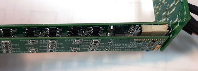