|
|
|
|
| AUG-22 | SEP-22 | OCT-22 | NOV-22 | |
| DEC-22 |
| JAN-23 | FEB-23 | MAR-23 | APR-23 | |
| MAY-23 | JUN-23 | JUL-23 | AUG-23 | |
| OCT-23 | NOV-23 | DEC-23 |
| JAN-24 | FEB-24 |
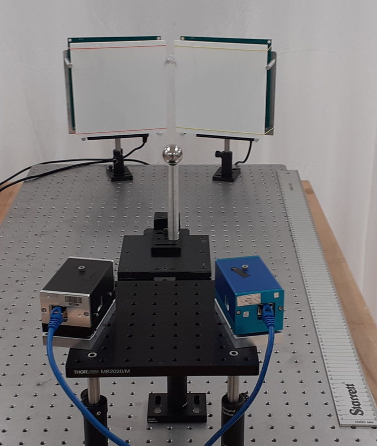
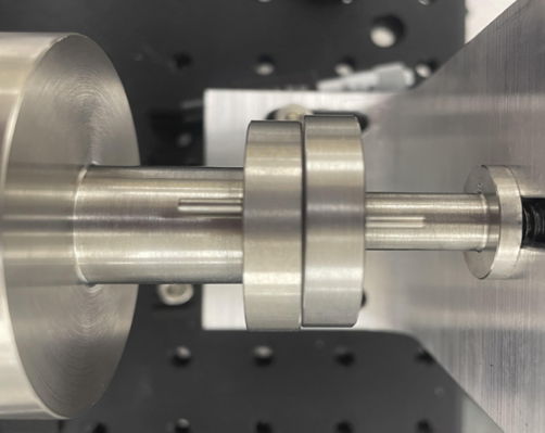
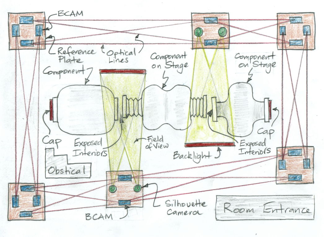
[05-FEB-24] We have completed our study of a prototype CPMS with a 50-cm operating range. The CPMS consists of two Silhouette Cameras (SCAMs) looking at a mockup of two steel flanges at range 40-60 cm. We have two backlights at range 100 cm, one for each of the SCAMs. The backlights are made of white glass illuminated from behind by an array of infra-red LEDs. The field of view of our SCAMs is 15 cm square at range 100 cm, so each SCAM's field is fully-covered by our backlight. The SCAMs are equipped with infra-red only filters, so they do not see reflections of our overhead lights.
When we want to take a silhouette image, we clear the image sensor, flash the backlight, and read out the image sensor. The process is managed by our Long-Wire Data Acquisition (LWDAQ) software and hardware. Our global coordinate system for these measurements has its origin on the SCAM mounting plate, with y vertical, z along the length of the CPMS, and x towards the left. We determine the actual position and orientation of target objects and SCAMs within our CPMS coordinate system with our Coordinate Measuring Machine (CMM), which is accurate to better than ±10 μm over its 1.5-m diameter range.
Our image analysis measures disagreement between the actual silhouette and an expected silhouette given a particular position and orientation of our target bodies. Each independent target body has its own model. Each body model we construct out of spheres, cylinders and conical shafts.
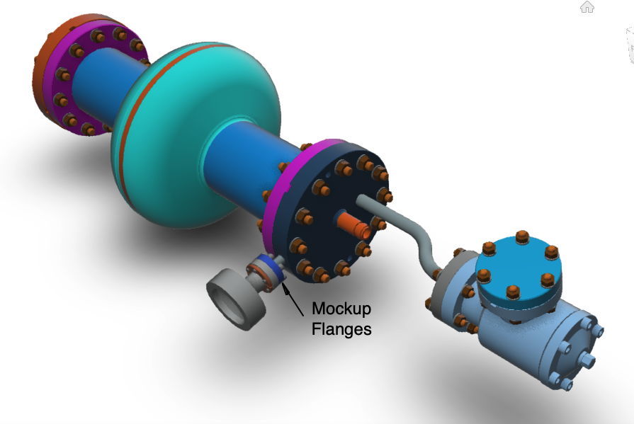
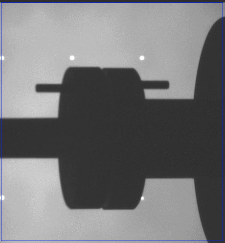
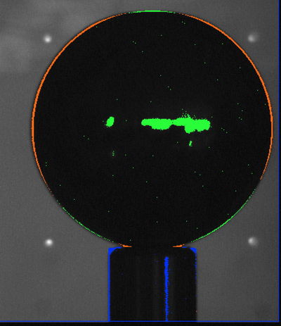
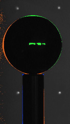
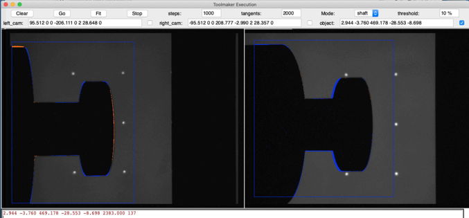
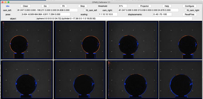
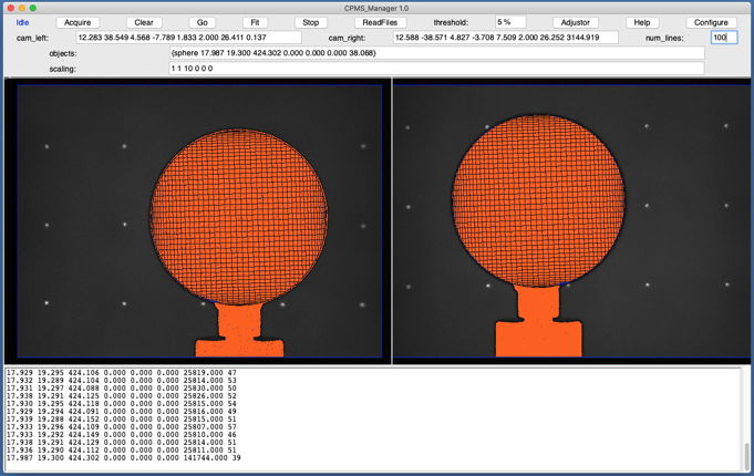
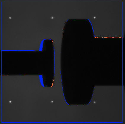
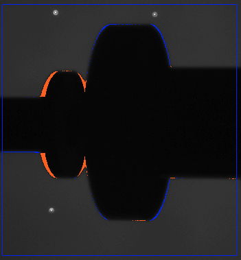
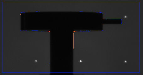
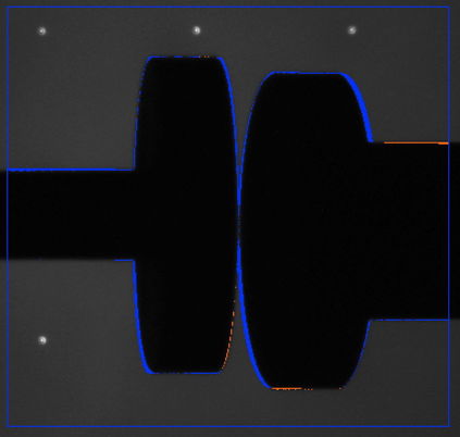
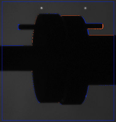
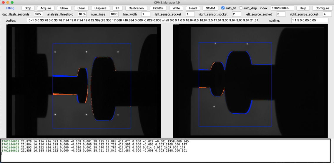
To test the performance of the CPMS, we use a stainless steel replica of the side port taken from the above model. We attach an alignment pin to each flange so that the CPMS can measure the rotation of the flanges about their axes. We see silhouettes of the flanges with pins below, as displayed during analysis by our CPMS Manager tool. The left image is from the left SCAM, the other from the right SCAM. We have selected a region in each image to use for our fit, so that we exclude parts of the silhouette that we have not added to our model.
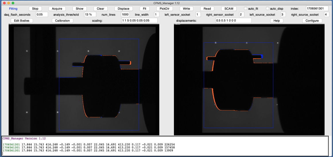
The CPMS measures the position of its target bodies by minimizing the disagreement between the silhouettes and the model projections. Imperfections in the image, such as the reflections of our windows and the bright spots on the backlight, have little effect on our measurements because they rarely arise on the perimeter of the silhouettes. Our error in measuring the separation of our flanges at range 50 cm is 50 μm rms in x and y, and 300 μm in z. The dominant source of error in the measurement is the fitting algorithm itself. If we take the average of eight measurements, our error drops to below 25 μm in x and y, and below 150 μm in z. With objects at range 100 cm, we expect our error to double. Our analysis today is slow. It takes roughly forty seconds to make one measurement of the two flanges with pins. With a more efficient model projection algorithm, such as those used in CAD proprams, our analysis will be ten times faster, at which point we can repeat the analysis several times per image and so reduce the error due to the fit. As it is now, we can run the fit ten times in about three minutes to obtain accuracy 25 μm in x and y, 150 μm in z at range 50 cm.
[31-AUG-22] We set up an array of nine infrared light-emitting diodes (LEDs). The nine LEDs are mounted on an ATLAS circuit called the Proximity Mask Head (A2045). The LEDs are HSDL4400, emitting at 850 nm. The A2045 runs roughly 80 mA through the LEDs. Each flat-topped LED emits in a 110° (2.7 sr) cone with intensity 5 mW/sr. Total power output per LED is around 13 mW at a cost of 100 mW of electrical power. In front of the array we place a sheet of thin white card and in front of this an optical post.
We set up a Polar BCAM 1.5 m away from the post and use the BCAM Instrument to obtain silhouette images of the post. We use the WPS Instrument) to analyze these images. The WPS analysis splits the image into top and bottom halves and fits straight lines to the edges of the silhouette.
We translate the post perpendicular to its own axis and the axis of the BCAM camera in steps using our stage. We record the left and right edge positions we obtain from the top and bottom halves, fit straight lines, and plot the residuals for the top and bottom halves separately.
Standard deviation of residual over our 7.5-mm movement is a little less than 1 μm. Slope of image position versis stage is 65.0 μm/mm. The BCAM's pivot-ccd distance is 75 mm. The post is roughly 115 cm from the camera lens.
We enhance the BCAM Instrument so that it provides vertical edge-finding of the same type as when we configure the WPS Instrument with analysis_enable=3. That is, we pre-smooth the image, obtain the magnitude of horizontal intensity, and then apply edge-finding to the entire image. Now we have no need of the WPS Instrument. See here for details of BCAM analysis. To obtain, analyse, and sort edges from left to right, we set analysis_enable=5, analysis_num_spots to "2 2" for two spots sorted by increasing x. To determine the x-position the BCAM Instrument intersects the near-vertical line with a horizontal reference line. The reference line is analysis_reference_um microns from the top edge of the image sensor. The default value is zero, so we use the top edge of the image sensor. But a better value is half-way down the image sensor, for which analysis_reference_um=1220 for the TC255 and 1924 for the ICX424.
[06-SEP-22] Report on sources of error in measuring position of a post by Nathan Sayer is Wire Finding.
[13-SEP-22] Report on performance of various backlight arrangements by Nathan Sayer is Position of LEDs.
[20-SEP-22] Comparison of card, opal glass, and ground glass in Uniform Illumination.
[11-OCT-22] We are building a CPMS test stand that incorporates full-scale mock-up of one small flange taken from an example SRF string, a three-axis stage and a rotator stage. We are having the flange components machined out of steel and polished. Drawings and views are in our Drawings directory.
[09-NOV-22] Our calls to potential users of the CPMS at SRF cavity construction sites suggest that 20% of SRF cavity components fail quality control because of contamination. An SRF cavity's quality factor during resonance should be of order 1010. With contamination, Q drops by an order of magnitude. One in four cavities must be removed, cleaned, and installed again. Estimated cost is $20k each time this must be done, with delays of one or two weeks. It is not clear what fraction of these contaminations occur during the final assembly phase where a CPMS would be deployed. Assuming a CPMS could eliminate half of these contaminations, and considering a string of thirty cavities, the CPMS would save $60k per string assembly. One CPMS installation costing $50k would be justified by two string assemblies. With ten sites building SRF cavities, the market is around $500k. Fusion power is a far larger market, but its requirements are less clear. They need to know where their shiny components are, but the main reason they do not want anyone touching the parts is because the parts will be radioactive. It's not clear to us how radioactive the parts will be, nor how high dose rate will be during operation of the fusion reactor. Assuming we can place our cameras and backlights in places with less than 1000 Gy ionizing and less than 1013 1-MeV eq. n/cm2 fast neutron doses, we will be able to serve the fusion reactors during maintenance by guiding separation and re-alignment of shiny components. Unlike the SRF cavity alignment, the fusion system would require multiple installations of cameras, one for each pair of objects to be separated and re-joined. With hundreds of fusion reactors and dozens of CPMS per reactor, this potential market is hundreds of times larger than the SRF cavity market, but also ten times less certain.
We propose to price one CPMS for one pair of components at $50k. This system will be mobile, clean, and can be applied to a variety of highly-reflecting shapes. Maintenance of the system will be covered by an additional $5k/yr fee. Our original CPMS included a global coordinate system defined with reference plates and BCAMs, see here. Our conversations with potential users suggest that this global coordinate system is unnecessary. Alignment of the string into a straight line is a problem separate from assembly without contamination. When we remove the global grid, and allow the user to move a single CPMS stereo camera and backlight from one station to the next, we find we have a system that we can indeed construct for $50k.
[22-DEC-22] We are working on the layout of the A304601A backlight circuit board. The backlight will consists of an array of twenty-five infra-red LEDs HSDL-4400 behind a 200-mm square ground glass diffuser. We prepare a simulation of the light distribution across the diffuser. The simulation allows us to vary the number of rows of LEDs up and down from a central row, q, number of columns of LEDs, r, separation of LEDs and diffuser in millimeters, d, and LED grid pitch, a.
Our chief concern with the backlight is the gradient of intensity with position. With 20-mm separation of diffuser and LED array, we see rapid variation along each row of LEDs as we move from one LED to the next. With 50-mm separation, however, intensity varies only with proximity to the edge of the diffuser, and is gentle.
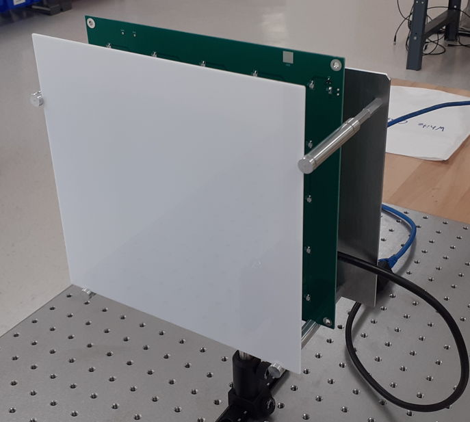
[18-JAN-23] We have our Infrared Backlight (A3046A) assembled, along with a holder for a 200-mm square glass diffuser.
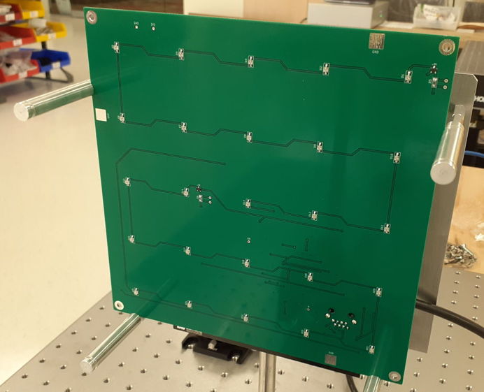
The A3046A is a LWDAQ Device that allows us to flash all twenty-five infrared LEDs at once, as well as two green indicator LEDs at the back. The A3046A is LWDAQ device type one (1), so we enter 1 for source_device_type in the BCAM Instrument when we take an image with the backlight. We have several varieties of ground glass and one type of white glass to load into the holder. Shown below is the white glass.
[01-FEB-23] We have a steel post in front of our 200-mm square A3046A backlight we measure its position with our edge-finding analysis. We vary exposure time and observe how the measured position of the left and right edges changes as the backlight becomes brighter.
As the backlight brightens, the edges move towards one another. White glass gives the more stable edge position. The movements are symmetric. The center line, calculated as the average of the two edge positions, does not appear to move at all as we increase the exposure from 1 to 100 ms.
[07-FEB-23] We try out the infrared backlight with ground glass and white glass. The variation in intensity with ground glass is greater than we expected from our simulation. The variation from white glass is far better, with the exception of bright points where the LED die itself is visible directly through the white glass.
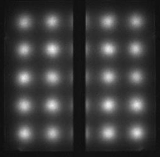
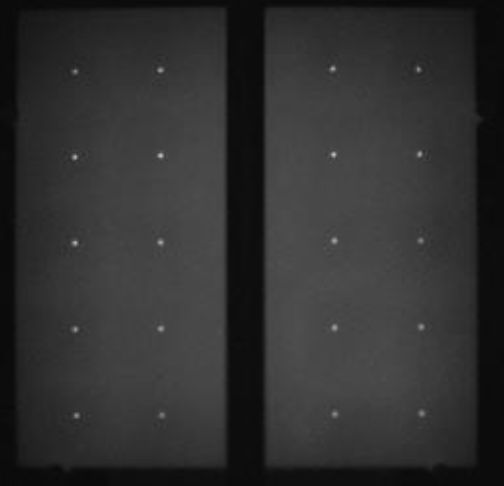
At first, the bright points seem like they will causes problems with our edge-finding. But it turns out that they have little or no effect. They are points occupying a few pixels, while the edges are lines occupying thousands of pixels. The magnification of our image is roughly 1/44. When we move the post 14 mm residuals to straight line fit on the image sensor are ≈1 μm for white glass and 2 μm for ground glass. We see systematic non-linearity for ground glass, not for white glass. For a full report see A3046A Initial Studies.
[20-MAR-23] We are working on code to project spheres and cylinders onto simulated image sensors. In a console-only test, we generate the following view of three spheres and a cylinder projected onto a 40 x 20 image sensor.
 --------------------------------------------------------------------------------
|          SSSSSSSSSS                                CCCCCCCCCCCCCC              |
|        SSSSSSSSSSSSSS                            CCCCCCCCCCCCCC                |
|      SSSSSSSSSSSSSSSSSS                        CCCCCCCCCCCCCC                  |
|      SSSSSSSSSSSSSSSSSS                      CCCCCCCCCCCCCC                    |
|      SSSSSSSSSSSSSSSSSS                    CCCCCCCCCCCCCC                      |
|      SSSSSSSSSSSSSSSSSS                  CCCCCCCCCCCCCC                        |
|      SSSSSSSSSSSSSSSSSS                CCCCCCCCCCCCCC                          |
|      SSSSSSSSSSSSSSSSSS              CCCCCCCCCCCCCC                            |
|        SSSSSSSSSSSSSS              CCCCCCCCCCCCCC                              |
|          SSSSSSSSSS                  CCCCCCCCCC                                |
|                                        CCCCCC                                  |
|                                      SSSS                                      |
|                                    SSSSSSSS                                    |
|                                    SSSSSSSS                                    |
|                                    SSSSSSSS                                    |
|                          SSSSSSSS  SSSSSSSS                                    |
|                      SSSSSSSSSSSSSSSS                                          |
|                      SSSSSSSSSSSSSSSS                                          |
|                    SSSSSSSSSSSSSSSSSSSS                                        |
|                    SSSSSSSSSSSSSSSSSSSS                                        |
 --------------------------------------------------------------------------------
[22-MAR-23] We have stereo cameras set up a rod and sphere in front of our backlight. We have infra-red only filters over each lens. But we break our white glass diffuser. We order a replacement. We refer to the silhouette cameras as "SCAMs" (pronounced "S-CAM"), similar to "BCAMs" (pronounced "B-CAM"). Our existing SCAMs are on optical posts. They use the ICX424 monochrome image sensor. We read them out using the BCAM Instrument. We use the BCAM coordinate transform routines. Ultimately, our SCAMs will mount on ball triplets identical to BCAM mounts. We have a new Pascal unit scam.pas containing the projection routines, and a new LWDAQ command lwdaq_scam that makes the routines available to LWDAQ. The following script projects two sphere and two cylinders onto one of our SCAM images.
LWDAQ_open BCAM
LWDAQ_acquire BCAM
set img $LWDAQ_config_BCAM(memory_name)
set camera "test 0 0 0 0 0 2 25 0"
set sphere "cylinder 0 0 1000 0 -0.04 -1 10 500\
	sphere 50 50 1000 20\
	sphere 50 -50 1000 20\
	cylinder -200 100 4000 0.1 0.1 1 30 1000"
lwdaq_scam $img project $camera $sphere
lwdaq_draw $img bcam_photo -intensify exact
The image we obtain with the above code is shown below. We are working in mount coordinate, which we also call SCAM coordinates. These are the coordinates defined by the three kinematic mounting balls. These balls do not exist yet, but our code is ready to support them. We place the spheres and cylinders in SCAM coordinates. We define a sphere with its center coordinates and radius. A cylinder we define as a point and a normal to one face, with the normal pointing into the cylinder. We have a radius of the face, and a length of they cylinder axis. By setting the length to zero we can define a circle in three-dimensional space.
[23-MAR-23] We start marking images to show which pixels are within a silhouette, and which are not. We color them orange if their intensity is equal to or below a threshold, and leave them untouched if they are above the threshold. We begin with an older image of a sphere with a threaded rod support.
In the above image, our orange silhouette is well-centered upon the actual sphere, and shows the detail of the screw threads. We take new images using two ground glass diffusers separated by 50 mm. These two diffusers give a backlight that is brighter at the center of our view than at the edges. We are waiting for our replacement white glass, which provides better uniformity. We start with the image from the left-hand camera. We see a horizontal line of small, bright rectangles near the center of the sphere. These are reflections of our office windows, through which the infrared light of the sun was shining.
Here is the simultaneous view from the right camera. The images show the importance of uniform background intensity. With a threshold intensity half-way from the minimum to the maximum intensity in the image, we get a superb isolation of the exact shape of our combined post and sphere, but the outskirts of the image are classified as silhouette also. No doubt we can figure out how to ignore these peripheral pixels, but we would rather start with a perfect image.
[24-MAR-23] We receive and install our white glass. We take 10-ms images with various infra-red pass filters to compare how well they reject our background light. Original images are here. Our plastic filters give poor rejection. Our Thorlabs FGL830M and Edmund Optics 13037 give good rejection. We place an FGL780M and FGL830M over our left and right cameras respectively and take two 20-ms images of sphere and post: Left.gif and Right.gif. Bright dots are the LEDs shining straight through the glass, and are a feature of our backlight. The bright dots do not confuse our silhouette classifier, but they allow us to measure the range of the backlight. Our classification routine now turns the overlay clear when our image agrees with our projection. Where the classifier sees silhouette and a projected object, or when it sees background and no projected object, it clears the overlay. Otherwise is assigns a color to the overlay. The number of colored pixels is a measure of the disagreement between the projected objects and the real objects. We attach a cylinder of diameter 12.8 mm to a sphere of diameter 34.8 mm and project them onto our left camera image.
The simulated objects are actual size. In the view of the camera, the SCAM x-coordinate is to the left, y is up, and z is away. We adjust the location of the post and sphere until we minimize the number of pixels that show disagreement. We assess the disagreement by eye. We find we can see movement of 50 μm in x and y, 1 mm in z. We place the center of the sphere at (−2.6 mm, −4.35 mm, 520 mm). We measure the distance from the post to the camera lens and find it to be 52 cm. With the a Toolmaker script you will find here, we scan the position of the object in x, y, and z and count the number of pixels at which the image and projection disagree.
When we move in z, we obtain the following plot, from which we conclude that a better value for the z-coordinate would be 517 mm.
If we use the whole-valued disagreement as our error function for a fitting routine, we will get the x and y coordinates with precision better than 100 μm rms, and z to better than 1 mm rms. Our stereo cameras are separated by 200 mm, which subtends and angle of 22° at the object. If the object moves 10 mm in the z-direction of the left camera, it will move 3.7 mm in the x-direction of the right camera. If our precision is 100 μm in x, our precision in z will be 270 μm in z. By using a real-valued disagreement measure, which includes information about the intensity of the original image, we should be able to improve our precision.
We find that projecting the sphere takes 90 ms and projecting the cylinder takes 720 ms. If we were to move this object in three dimensions with a simplex fitter, we would need one second per step. Assuming we start the fit with a good estimate of position, the fit will take around a 30 s per camera, or one minute for both. For more complex objects, the fit time could easily approach ten minutes. We need to write a more efficient projection routine, so as to speed up this analysis by one or two orders of magnitude.
We set up our simplex fitter to minimize our silhouette disagreement, and improve its reporting features, so we can watch the fit in progress, see lwdaq_simplex. We choose a starting position with projection and silhouette overlapping by about 50%. The fit takes one second per step. After one hundred steps, we have converged to (-2.67 -4.314 517.3) with disagreement 3607 pixels. This minimum is less than the one we found by eye. We start from a different position and converge to (-2.66 -4.35 517.1) with disagreement 3610 pixels. Another one and we see convergence after 60 steps to (-2.65 -4.37 517.1) and disagreement of 3606 pixels. The fit appears to have precision 10 μm in x and y, and 100 μm in z.
[31-MAR-23] Our current SCAM lenses are consumer M12 NOIR surveillance camera assemblies with 25-mm focal length. Note that NOIR is short for "no infra-red blocking filter", which means "yes infrared". The back side is a 10-mm aperture within the M12 case. We reduce the aperture to 3.7 mm with washers we glue to the back side of the lens. We place our 200-mm square backlight 90 cm from our stereo SCAM and focus the SCAM on the points in the backlight. We place our 34.8-mm sphere and 12.8-mm diameter post as close as we can to the backlight glass. The sphere is at range 88 cm. We take a 50-ms exposure and obtain a this image.
Reflection of the backlight in the surface of the sphere is clearly visible all around the perimeter of the sphere image. The band of reflection is thicker on the right side because we are using the right-side SCAM. In order to classify the entire silhouette of the sphere and cylinder correctly, we must increase our intensity threshold from "20 %" to "50 %". The code "50 %" means the threshold is 50% of the way from the minimum intensity in the analysis boundaries to the maximum intensity in the same boundaries. With this elevated threshold, roughly 80k pixels at the edges of the backlight are classified as silhouette. But this 80k remains fixed as our fitter moves the simulated body around, so that our fit converges without difficulty.
We move our post and sphere from range 88 cm to 62 cm and obtain this image with the left-hand SCAM. The edge reflections is still present around the perimeter of post and sphere. Blurring of the image by defocus is hi-lighted by the appearance of one of the backlight LED points within the left side of the post silhouette.


The defocus makes our measurement of the silhouette perimeter sensitive to our choice of classification threshold. We select a portion of the post edge and increase threshold from "5 %" to "90 %" to demonstrate this effect.


We apply our "50 %" threshold to classify the pixels. We have a total of 61k silhouette pixels. A small fraction of these are in the silhouette itself. Most are distributed around the edges of the backlight. We call these peripheral silhouette pixels the "halo". Provided that the halo does not intersect with the set of projected pixels, nor touch our image silhouette, it will have no effect upon our analysis. The number of halo pixels in any given image is fixed. We apply our fitting routine. We represent the result below. As we increase the threshold, the post silhouette will widen, suggesting that the post is closer to the SCAM. Defocus introduces a systematic error in our measurement of the object z-coordinate. Depending upon our choice of threshold, the object will appear closer or farther away.
We scan the position of our simulated body in x and y to see how the disagreement varies with position in the presence of defocus. We use "50 %" for our threshold.
In a defocused image, our binary classification results in a disagreement value that no longer provides a clearly-defined minimum at any particular value of x or y. Nevertheless, we are still able to obtain precision of 100 μm rms, compared to 50 μm rms in a sharply-focused image. We move our object to range 75 cm and adjust the lens to obtain a sharp image 75cm.gif. We move to 88 cm and 58 cm and obtain 75cm.gif and 58cm.gif respectively. We scan in x for each image. We use threshold "40 %" for the 58-cm image or else the halo touches our sphere. We use "40 %" in the 75-cm image as well. We must use "50 %" in the 88-cm image or else the edge reflections ruin our silhouette. Because the halo varies from one image to the other, but is fixed for any given image, we plot the disagreement minus the halo.
The defocus is most pronounced in the 58-cm image, for which the range is 23% shorter than the focal range, compared to only 17% longer at 88 cm. Even in the sharply-focused 75-cm image, however, we see our disagreement minimum is poorly-defined.
[03-APR-23] We install new lenses in our SCAMs. We have 25-mm focal length plano-convex lenses, 6-mm diameter, Edmund Optics 37-777, with a 2.7-mm aperture made out of a steel washer. We mount these in M12 threaded holders. We now obtain sharp focus for ranges 60-85 cm. We take images from the left and right cameras at 60 cm, 70 cm, and 85 cm, see here. To obtain a bright, clear image, we use a 100 ms exposure. With a 10-ms exposure and strong intensification, however, the image still shows sharp contrast and focus, and our fit proceeds well.
[11-APR-23] We are thinking about how to measure the rotation of a flange about its cylindrical axis, so as to align bolt-holes. We figure we need some kind of fiducial.
The length of the fiducial pin could be half the radius of the flange, and at least √-1 times the radius. Our SCAMs see the pin and measure the altitude of its end with respect to the flange center-line with a precision of 200 μm, which in turn allows us to measure the orientation of the flange with precision 200 μm divided by the radius. A battery-powered infrared light is another idea, and we can place it on the horizontal to maximize precision. Both require that we add a fiducial mounting hole to the flange.
[14-APR-23] We submit our Phase II application 13862200.
[03-MAY-23] We have a new version of the backlight circuit A3046B. In our TS1 we have equipped our cameras with lens holders that are secured with screws rather than tape, and M12 adaptor and extender optics that allow us to focus any of our lenses and mount our infrared filters in a stable fashion. We resolve to make a second backlight and direct each camera to a separate backlight with the objects in the middle.
[10-MAY-23] We re-arrange our test stand for two backlights. We will call this arrangement the dual-backlight. The left-hand camera looks at the right-hand backlight. Our camera lenses have focal length 25 mm with 2.7-mm apertures. We model the camera as a pinhole aperture and a screen. The center of the pinhole is the pivot point of our camera. The pivot point will be close to the center of the aperture (see Appendix 1 here). We arrange the camera pivot points to be 100 mm from the axis of symmetry of our CPMS. The backlights are at 900 mm, with their inner edges almost touching and their outer edges almost 200 mm from the axis of symmetry. The backlights themselves are 200 mm square, but we orient them so that they are perpendicular to the axis of the camera that views them.
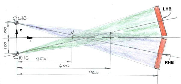
The CPMS coordinate origin we take to be the mid-point of the line between the two camera pivot points. The z-axis is along the line of symmetry, the x-axis is horizontal, and the y-axis is vertical. The LHC and RHC each have their own coordinate systems, which for now we will take to be referred to their pivot points, with the camera z-axis along the camera axis, and x-axis horizontal, y-axis vertical. So the camera z-axes are at 12.5° to the CPMS z-axis.
We have shaded the fields of view of the two cameras, which are just able to see the full width of the backlights. We find we can place our 34.8-mm diameter sphere anywhere from 350 mm to 600 mm from the cameras and see the entire sphere silhouette in both cameras. We call this interval the working range of the CPMS. We focus the camera on the sphere at the far range. The image is now sharp at the far range an slightly blurred at the near range. At the near range, however, we have greater precision because the object is bigger. With the left-hand camera we obtain near and far images and see how well we can fit our model to the image.
On the assumption that our pivot point is exactly 25 mm from our image sensor, our fitted ranges are 348 mm and 593 mm, while our measurement by ruler is 35 cm and 60 cm. The angle between the camera axes is 25°. Our uncertainty in measuring range will be only twice as great as our uncertainty in measuring position perpendicular to the axes. Our half-size CPMS is roughly one meter long, including the camera and backlight stands. A two-meter system would provide working range 70 cm to 120 cm and be two meters long.
[11-MAY-23] We set up two post-mounted spheres in the field of view of our LHC (left-hand camera). One is at roughly 70 cm range, the other at 45 cm. The one at 70 cm is fixed, the one at 45 cm we mount on a three-axis stage. Both spheres are 34.8 mm in diameter, mounted on 12.5-mm diameter posts.
We move the closer object in the CPMS x-direction in 1-mm steps. At each step we take an image withe the LHC and save it to disk as Sx.gif. We build a model of two post-mounted spheres that each can move independently, see here. We fit their positions to each silhouette image in turn, using thirty iterations for each, and continuing if the fit has not converged. Usually the fit has converged by 30 iterations, but not always. The 30 iterations take about three minutes. We now have measurements of position of both objects in LHC coordinates.
Because we know the diameter of the spheres and the width of the posts, the analysis adjusts the range of the objects until they fit with the 25-mm pivot-ccd distance we have specified for the cameras. The z-position is only as accurate as our 25-mm estimate of the pivot-ccd distance. But measurement of the displacement of the objects in the x-direction is independent of our error in pivot-ccd estimation. The analysis is comparing these displacements to the known dimensions of the object. Our error in x-displacement is proportional to our error in measuring the sphere and post. We expect our measurement of x displacement to be accurate. Given that the camera x-direction is at 12.5° to the CPMS x-direction, the slope of x-displacement with stage displacement should be cos(12.5°) = 0.976 mm/mm. We get 0.954 mm/mm.
The standard deviation of the x1 residuals is only 40 μm. The x2 residual for the stationary object is 95 μm. Our measurement of the stationary object is disturbed in several images by false silhouette pixels at the edge of the backlight. Our y-residuals are larger, we suspect because there is no sharp, straight edge to give us the y-position. The range residual 0.8 mm for the moving object and 1.5 mm for the stationary object.
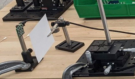
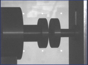
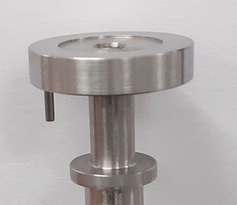
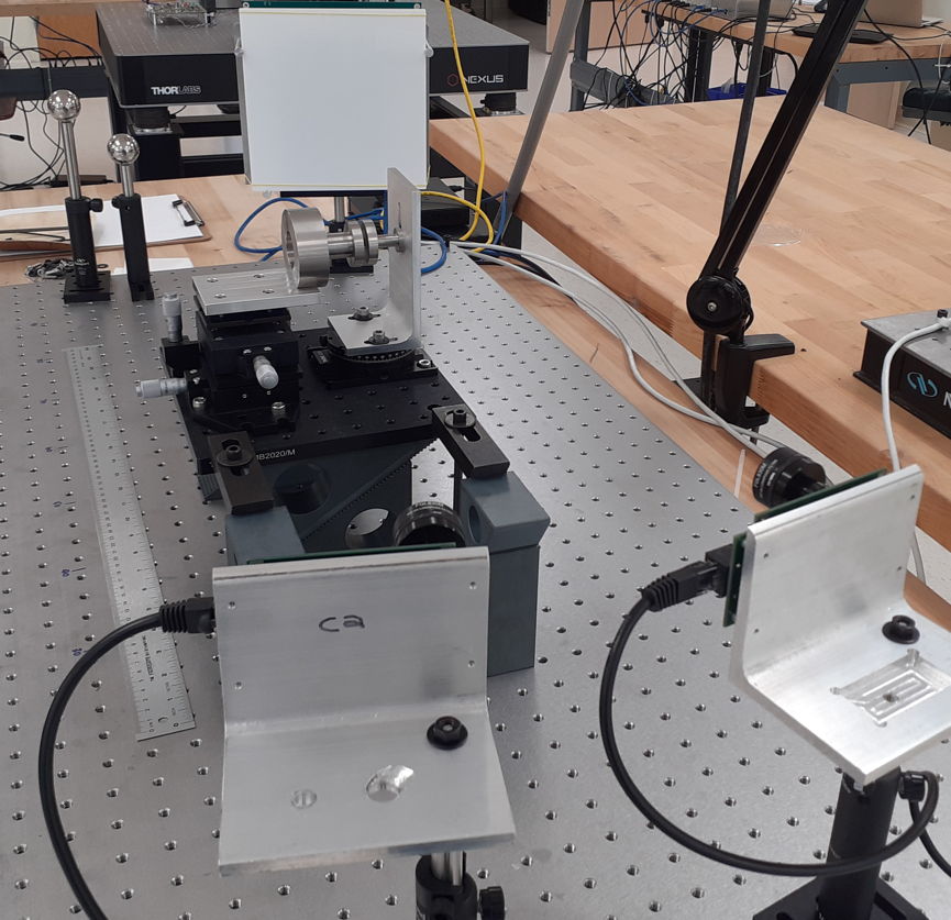
[15-MAY-23] We put together a two-flange mockup, as shown below, except that the three-axis stage is not mounted upon an optical rail, but screwed directly to the base. Both parts are made of stainless steel and have the same dimensions as an actual SRF cavity flange built at FNL. Machine shop drawings and views are in our Drawings directory.
Here are the dimensions of the two flanges, seen from the side. They are radially symmetric, but rotation about the vertical axis will cause a change in their apparent shape. We will implement each flange as a combination of three cylinders, and permit each to translate in three dimensions and to rotate about a vertical axis.
We view the mockup flanges with the LHC. We obtain a series of images 10mm.gif down to 0mm.gif, see here, as we move the CPMS x-direction micrometer ten millimeters, during which the separation of the two flanges drops from 10 mm to 0 mm. The micrometer is moving Flange One in the CPMS x-direction, which is close to the LHC x-direction.
We see desk lamps and other furniture reflected in the backlight glass, and reflections of our windows in the cylinders themselves. But these reflections do not affect the classification of the silhouette pixels. Only the reflection off the front edge of Flange Two's mounting bracket affects the classification, and this feature is far from our flange silhouettes.
[17-MAY-23] We complete clamping of our mockup flanges at the correct height for surveying and rotation, see here. We remove the right-hand flange from view and work with a portion of the left-hand flange. We allow the fit to rotate as well as translate the flange. We represent the flange with two coaxial cylinders. We reduce the amount of image we must project into by reducing the analysis bounds around the flange.
For the first time we realize that there are two orientations of the flange that will satisfy our silhouette: two rotations about the vertical axis. With two cameras, there will be only one rotation that satisfies both. When we start using two cameras, we will fit using both images at once. By hand we translate and rotate the modelled component. The disagreement changes significantly with 100-μm translations. We improve the disagreement measure so it scales the disagreement between zero and one depending upon how close the intensity is to the threshold.
[18-MAY-23] We enhance our analysis routine so it will accept a "spread" for the transition between silhouette and backlight intensity. The spread is a fraction between zero and one. We use it to multiply the difference between our threshold intensity and the minimum intensity in the image. The result is the "extent" of the transition between definitely silhouette and definitely backlight. An intensity less than threshold − extent is definitely silhouette, and an intensity greater than threshold + extent is definitely backlight. The presence of projection in a definite silhouette means zero disagreement. In the figure below we show how we obtain the disagreement between projection and silhouette using the extent and the threshold, depending upon whether the pixel is occupied by a projected object or not.
We scan our projection position in the y-direction and try a range of spread values to see how the spread affects the disagreement. We subtract the minimum disagreement from each plot so as to bring them all into the same range. Otherwise the disagreement for spread=0.5 is 9000 while that for spread=0.0 is 3000.
Our spread creates a real-valued disagreement function. For a high spread, we see some alleviation of the poor behavior of our error function, but no dramatic improvement.
[19-MAY-23] Our original object projection routines work by going through ever pixel in an image and seeing if the ray passing through the camera pivot point and the center of the pixel intersects the object. If so, we assume that the silhouette of the object would cover the pixel. For a cylinder, on a 1-GHz laptop, this calculation takes 2 μs. For a 400-kByte image it takes 800 ms. We now try starting with the object, tracing its outline on the image, and filling in the resultant shape. In the case of a sphere, we calculate tangents to the sphere that pass through the camera pivot point, and we rotate these about the line from the pivot point to the center of the sphere, so as to create a set of points around the perimeter of the projection.
[01-JUN-23] Our outline projection routine allows us to specify a number of points around the circumference of a cylinder or sphere. We project these onto our image sensor and join them with lines in various ways. With enough points, the lines fill in the object entirely.
The outline projection gives a reliable fill with one thousand points. In Projector.tcl we have a Toolmaker script that draws a projected sphere, cylinder, or flange with pin. The program allows us to rotate and translate the object with sliders. The projection with one thousand points is fast enough that we can rotate the object as fast as we like.
[07-JUN-23] We are using our outline projection as the basis of our comparison of the silhouette and projection. We are working with Left_Flange obtained 17-MAY-23. We make numerous, substantial improvements to our simplex fitting routine. We can now accommodate varying sensitivity to coordinates with a scaling of the simplex construction vertices. We can set the start size. We can set the number of restarts, which is where we re-construct the simplex when we appear to be getting stuck. We enable shrinking the simplex after we are done restarting. The convergence criterion is simplified: when we shrink the simplex below the end size, we are done. We abandon our spread disagreement function, reverting to a routine that simply counts disagreement pixels. We are using 1000 projection points. With two restarts, our fit now converges automatically in about fifteen seconds. We fit from a variety of starting points and obtain the following end values.
In our fit, we are adjusting the x, y, and z position. We are rotating the flange about y and z, but not about x, because it starts with its axis parallel to x and rotation about x does nothing to a symmetric cylinder. We have 20-μm resolution in x and y, 400 μm resolution in z.
Our image provides us with two error minima. One where the y-rotation is −157 mrad, one where the y-rotation is +205 mrad. To the first approximate, the two are the same: we cannot tell which way the cylinder rotates about the y-axis. But our fit is now so precise that it can tell the difference between the two because of the effect of range. The end of the cylinder that is closer will be larger. With the correct rotation, our error is around 280, and with the incorrect rotation, it is around 560.
[08-JUN-23] The ambiguity in y-rotation does not exist if we view the flange with two cameras. We have left and right cameras running, along with left and right backlights. We run our fit with left and right silhouette images.
Our fit does not converge if we hard-code the camera constants. Instead, we fix only the pivot position of the left camera at "-90 0 0". We allow the left camera axis direction, pivot-ccd, and sensor rotation to vary, as well as all parameters of the right camera, and the position and orientation of the flange. We are now fitting with sixteen parameters: four for the left camera, seven for the right camera, and five for the flange. The fit converges every time. From a poor starting position, it takes one minute, with roughly 300 iterations. But this fit is under-constrained, and so does not converge to the same value every time.
With too many free parameters, our x-resolution has degraded from 20 μm to 1 mm.
[11-JUN-23] We can now turn on and off fitting of left camera, right camera, and object parameters. For the cameras, we are taking the line joining their pivot points as z=0, and the half-way point along this line as our CPMS coordinate origin, with x parallel to the line and y completing our coordinate system. When we fit one or both cameras, we are adjusting the separation of the pivot points along the x-axis. For each camera we fit the camera axis direction and ccd-pivot distance. We refrain from fitting the rotation of the image sensor for now. The camera axis directions are going to be around ±220 mrad in x. We correct a long-standing assumption in our BCAM routines, whereby the the z-component of the camera axis always unity. This change causes our measurement of the separation of the cameras to increase by 2 mm.
When we fit the calibration constants of both cameras, as well as the object position, using our two images, we see the fit converge to a range of locations with disagreements from 616 to 1362. We pick the camera calibration constants that give disagreement 616, turn off left and right camera fitting, and fit only object position.
With fixed camera calibration constants, our precision appears to be 10 μm in x, 40 μm in y, and 170 μm in z. We note a consistent failure of the fit to match the left side of the flange in the left image, see below.
The blue pixels show where our projection draws the sharp edge of our modelled flange. But the actual flange is finished with a chamfer, and our left camera has a clear view of the chamfer.
[15-JUN-23] A new shaft object provides a sequence of radii along an axis, with axial lines between the faces. We can use the shaft object to project cones and chamfers. We start by creating a three-face shaft to match our flange, ignoring the chamfers. Our Fitter.tcl program allows us to switch between a three-cylinder implementation of the flange and our shaft implementation. The cylinder implementation with zero tangents reverts to our original, slow, complete-image projection method. We compare the three projetions and find them in close agreement.
Our Projector.tcl program now provides a shaft projection we can rotate and translate.
[21-JUN-23] We enhance our simplex fitter so it can refrain from fitting parameters for which we set the scaling factor to zero. When we have N parameters and we choose M<N to fit, the simplex consists of N+1 vertices of which M+1 are duplicates. The fitter treats them as one vertex, and so fits in M dimensions while working with N+1 parameters. We can now turn off fitting of individual parameters by setting their scaling factor to zero. Fitting only the shaft object, the three cylinders, we obtain resolution better than 100 μm rms in x and y.
[23-JUN-23] We have two Black SCAMs on our stand, equipped with 25-mm plano-convex lenses and 2-mm apertures. The SCAMs are assembled in two modified Black D-BCAM Chassis, scam_base_black. For photograph of test stand see Mockup_and_SCAMs.jpg. We focus at 40 cm, see RC_FR_40cm.gif and at 90 cm, see RC_FR_90cm.gif. We focus both at 40 cm and take new images for fitting, including both flanges of our mockup.
We fit 6 camera parameters and 5 flange parameters. The fit concludes that the two pivot points are separated by 189 mm, but our measurement shows 167 mm. We have two images of the flange, and each image gives us an x-y position, an x width and a y width. We have 2 × 4 = 8 measurements and 11 unknown parameters. We freeze the x-positions of the two cameras, and obtain better results, although we still are fitting ten parameters with only eight measurements.
left_cam "83.500 0.000 0.000 -198.708 0.000 2.000 24.875 0.000"
right_cam "-83.5 0 0 200.273 1.157 2 24.300 0"
The fit concludes that the pivot-ccd distance is 24.3 mm for the second camera, but we measure it to be closer to 27 mm. With three spheres instead of the flange, we would have enough information to calibrate the cameras. For now, however, we measure resolution by turning off camera parameter fitting and starting from arbitrary flange positions and fitting.
[27-JUN-23] We glue 12.5-mm diameter 830-nm longpass filters over our lenses. We rotate our stand so that the cameras face our bright windows, but their view is blocked by the backlights. We no longer see reflections of our windows in the backlight glass. Camera cone balls are separated by 170 mm. Apertures separated by roughly 167 mm as before. Images here.
[02-JUL-23] We create the CPMS Calibrator tool for our LWDAQ software. The main tool window currently provides our fitting program. The Projector button opens a projection window. The projector shows the projection of the object defined in the calibrator, as seen by the two cameras defined in the calibrator.
[03-JUL-23] We enhance our CPMS Calibrator so that it reads and displays four pairs of images taken with our calibration sphere in for different positions along a straight line. We assume the sphere moves in a straight line, and that the distance along the straight line, as given by our 10-cm micrometer stage, are correct. We measure the diameter of the sphere with calipers. The locus of the sphere has a start point and a direction in the CPMS coordinates. The direction is two rotations, the start point is three coordinates. The sphere locus presents us with five unknowns. We fit the camera parameters and object parameters repeatedly. We are fixing the camera pivot x-positions to be symmetric about zero. We are setting the camera pivot y and z to zero. The left camera y-axis we set to zero, but right camera y-axis can vary. We are fitting CCD rotation for the first time. We have eight camera calibration parameters.
We have three measurements per image: x, y, and diameter. With eight images, that's 24 measurements. We have 8 camera unknowns and 5 object unknowns, 13 unknowns in all. Our resolution is superb in y, but in x and z it is poor. We fix the camera calibration constants and fit only the five object parameters.
We have 24 measurements and only 5 unknowns. Our fit is severely constrained. Convergence takes between thirty seconds and one minute, 90 to 180 iterations. We obtain 100-μm precision in X and Z, 25-μm precision in Y.
[04-JUL-23] We suppress fitting of the rotation of our image sensors. We add a post to each sphere, to complete our silhouette matching.
We fit the object position with spheres only, then fit with sphere and post, and find that the two agree to within tens of microns in X, Y, and Z. The fitting with the posts added is three times slower than with the spheres only. Our cylinder projection routine is inefficient.
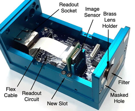
[13-JUL-23] We have built our first Blue SCAM, to complete our symmetric stereo SCAM pair for our half-sized CPMS. The infra-red only filter is 12.5-mm diameter, 830-nm Edmund 18-895, glued to the front of our brass lens holder. In the brass holder is a 6-mm diameter plano convex lens with focal length 25 mm, Edmund 37-777. The SCAM is constructed out of a modified D-BCAM chassis. We have cut an extra mounting position for the image sensor, to suit the 25-mm focal length. We have masked holes in the chassis that would otherwise be used for lasers and laser board mounting screws. We install our Blue SCAM in our half-sized CPMS, see photograph.
[30-AUG-23] We order a FARO Technologies measurement arm, model ARM-0040-4FA. Its operating range is a diameter of 1.5 m. Its absolute accuracy in that range is specified as ±12 μm. We will refer to this instrument as our coordinate measurement machine, or CMM. With our CMM, we will measure the position of highly reflecting objects directly, so as to permit calibration of our SCAMs. Once we have calibrated SCAMs successfully, we can measure the position of objects with both SCAMs and our CMM so as to determine the accuracy and resolution of the CPMS.
SEP-23
[20-SEP-23] We have received and unpacked our CMM. We are learning how to use it, measuring spheres and defining coordinate systems. The software that comes with the CMM has been able to read in solid models of our flanges, so that it can measure their position and orientation directly with knowledge of the model.
[06-OCT-23] We have an SCAM mount, which is identical to a BCAM mount defining a global coordinate system for our optical table. We mount a 1.5" diameter steel sphere on a post on our micrometer stage. We move 100 mm in 10-mm steps. The movement of the stage is approximately parallel to the global z-axis, and in the negative direction. At each position, we measure the sphere position.
Residuals to straight line fit in z are roughly 5 μm rms and include the error in adjusting the stage. The residuals in x, which is parallel to the table and perpendicular to the movement, are around 2 μm rms. We are able to measure all around the sphere in the x and z directions. Residuals in y are closer to 5 μm. To obtain the y-coordinate, we note that the CMM must subtract its measurement of radius from its measurement of the top side of the sphere to obtain the center position because we are unable to touch the bottom side of the sphere where it is mounted to the bolt.
[16-OCT-23] We define a global coordinate system with a dedicated three-ball mount. We measure the three balls of a left and right SCAM mounts with our CMM. We mount a black SCAM on the left and a blue SCAM on the right. They look down our optical table to their backlights. We move our 1.5" sphere to four positions spanning 100 mm. In each position, we take images from two SCAMs and measure the location of the sphere with our CMM. We update our CPMS Calibrator tool, producing V2.1. The new version reads a text file produced by the CMM to obtain the mount coordinates and sphere positions. It reads the left and right SCAM images of the sphere in its four positions. We equip the program with the default values for calibration constants of black and blue SCAMs. When we press Fit, the program adjusts the calibration constants of both cameras until it minimizes the disagreement between image and projection. Having done this, we fix all constants except the pivot x and y. These we vary and re-fit, obtaining ten fits from various starting points.
Our resolution is better than 20 μm. The average values for both cameras are within a fraction of a millimeter of the nominal values we obtain from the camera chassis. When we allow all constants to vary, we find that we can always obtain a good fit, but the calibration constants are not well constrained. In order to constrain the longitudinal parameters, we need a greater variation in range of our sphere. But any of these sets of calibration constants are likely to be equally accurate for the ranges covered by our sphere positions.
[23-OCT-23] We prepare a new LWDAQ Instrument, the SCAM. It takes images form SCAMs and applies a threshold, colors the silhouette pixels in orange. We prepare a new LWDAQ Tool, the CPMS Manager. It uses the SCAM Instrument to acquire two images, one from a left-hand SCAM, another from a right-hand SCAM, both mounted on a calibrated CPMS plate. We include in the CPMS Manager the coordinates of the mounting balls, and the calibration constants of the cameras. The former we obtain from our CMM, the latter from our CPMS Calibrator. The CPMS Manager acquires images and fits an object to the silhouette. We can specify the number of lines we use to fill the modelled object. We have been using 2000 lines to make sure our spheres and cylinders are filled completely. We now find that the result of the fit is not a strong function of the number of lines we use.
We fit repeatedly from the same starting point, each time increasing the number of lines and measuring the execution time. We plot the deviation in global x, y, and z position we obtain from our fits versus number of lines.
For more than thirty lines, our x coordinate is stable to 30 μm rms, y to 10 μm rms, and z to 120 μm rms. It now appears that we do not have to work upon a perfect, fast, fill algorithm for our shapes. We can render them with a hundred lines, which is fast.
[31-OCT-23] We move our sphere in x, y, and z. We measure the sphere position with our CMM and with our CPMS. Our measurements are absolute measurements with respect to the CPMS plate's coordinate system. We have our measurement of the CPMS plate, made earlier by the CMM, and we have our calibration of the two SCAMs, produced from an earlier measurement with the sphere in four positions. We start with a 10-cm movement in Z
The intercept in x is 0.15 mm, suggesting an absolute accuracy in x of order 0.1 mm rms. The intercept in z is −2.3 mm. The following plots show the residual to a straight line fit in z and x, both of which are horizontal.
We mount our sphere upon a vertical translation stage, which permits us to move it by a few millimeters. Intercept in y is −0.2 mm. We obtain the following residuals.
[06-NOV-23] We adjust exposure time while measuring the position of a 1.5" sphere with our CPMS. We are using absolute intensity threshold sixty ADC counts, which we obtain by setting the threshold string to "60". The SCAM Instrument implements the same set of threshold codes as the BCAM Instrument.
Detail of 120-220 ms exposure below. Our x and y measurements are stable to around 50 μm rms over this range, and z is stable to around 100 μm rms.
We take a 170-ms image and increase the silhouette intensity threshold from 40 to 80 ADC counts absolute. We obtain the CPMS measurement of sphere position for each threshold value.
As we increase the threshold, more pixels are included in the silhouette. The sphere grows larger. Our CPMS fit moves its model of the sphere closer to the SCAMs so that the modelled sphere will grow to match the silhouette. Closer to the SCAMs is a lower value of global z-coordinate. The sphere has to move in the global x and y as well, so that it remains centered upon the silhouette. As we increase the threshold, the z-coordinate of our measurement drops by roughly 0.15 mm/cnt. Our x and y measurements change by roughly 20 20 μm/cnt.
[07-NOV-23] We take a 170-ms image with the blind drawn, which we call "dark". We see no reflections off the surface of our sphere. We take another with the blinds open, which we call "light". We see reflections of sunlight in both sides of the sphere. We measure
We fix our threshold at 60 cnt and vary the exposure time. For each exposure we measure x-coordinate with the CPMS. We plot deviations from the x-coordinate at exposure time 170 ms.
In the detail around our favored operating threshold, we see that the x-position drops by 0.5 μm/ms with increasing exposure with the sunlight blocked, but behaves chaotically over a range of ±200 μm with the sunlight reflecting off our sphere.
[08-NOV-23] We operate the CPMS in what we believe is it's optimal state: threshold 60 cnt, exposure 170 ms, window blinds closed. We place the sphere at global z = 495 mm and translate with a stage in the positive x-direction. We obtain the CPMS measurement error for each sphere position, which is the difference between the CPMS measurement and the CMM measurement of the sphere position. We plot error versus stage position.
We are moving in x, so our x-coordinate has a slope error of +0.01 mm/mm, or +1%. The error in z is +0.6 mm, which would cause a slope error of 0.12% at range 495 mm, but not 1%. We rotate our stage and move 100 mm in the positive global z-direction.
[20-NOV-23] Nathan writes. "Today we compared the new CPMS backlight with the old. The new backlight puts about 70mA through each chain of LEDs compared to the 15mA that ran through each chain on the old backlight. We used the SCAM instrument along with the Camera instrument in order to measure the contrast of each image. We took one image with the old backlight at an exposure time of 170 ms. This image had a minimum intensity of 50 counts and a maximum intensity of 200 counts, giving us a contrast of 150 counts. We then swap to the new backlight and adjust the exposure time until we reach a similar contrast at 150 counts. The exposure time required to reach that same contrast was 48ms, roughly 28% of the exposure time required to achieve the same contrast with the old backlight."
[22-NOV-23] We have three backlights, which we number No1, No2, and No3. Nathan reports that all three have been modified to deliver 70 mA, but two of them are not tested. We use our new Camera Saturator tool to measure the maximum and minimum intensity in SCAM images as we increase exposure time, and we do so for all three backlights.
At zero flash time the apparent contrast is non-zero because of noise in the image. Above zero, the contrast is linear with flash time until we reach pixel saturation, which starts to occur at 50 ms for No1, 80 ms for No2, and 200 ms for No3. With the brightest backlight, we obtain perfectly adequate images at exposure time 20 ms.
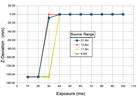
[29-NOV-23] With our brighter backlights, we compare two rules for selecting the silhouette intensity threshold. In "10 %" we set the threshold 10% of the way from the minimum to the maximum intensity in the image. With "5 %" we set it 5% of the way. See BCAM Instrument for the various options we have for selecting the threshold in an image. We place our sphere at roughly 450 mm from our CPMS. We increase exposure time from 10 ms to 180 ms and measure the deviation in x, y, and z. We find that "10 %" produces a more stable measurement.
As we increase the exposure time, the silhouette appears to shrink, and our CPMS judges it to be farther away. Its z-position increases.
We choose 40 ms and "10 %" as our optimum exposure time and threshold. For these values, we can halve or double the exposure time and obtain the same x, y, and z to within a few microns.
[30-NOV-23] We discover an oversight in our definition of the CPMS global coordinate system within our CMM program. We correct the bug. The three 1/4" precision reference balls are now in the y=0 plane, which is correct. We perform a fresh calibration. The CMM output file and the eight images we obtain of the sphere in four positions seen by both SCAMs are all here. When overlaying the modelled sphere on our silhouette images, our CPMS Calibrator and Manager allow us to specify the number and width of the lines that represent the sphere. We use width 1 px (one pixel) and 2000 lines to provide an exact fill.
As we repeat the fit from various random starting camera calibration constants, we see pivot.z varying from -20 to +7 mm. But we know from construction that the lens holder protrudes by 0.5 mm from the face of the SCAM, the aperture is 2.5 mm into the lens holder, and the cone ball lies 6.0 mm behind the face. So pivot.z is roughly 6.0 + 0.5 - 2.5 = 4.0 mm. We fix pivot.z at +4.0 mm and run our fit. We use our fitted SCAM calibration constants in our CPMS Manager, along with the SCAM mount measurements from the CMM, to measure the position of the calibration spheres. We compare to the CMM measurement of these same spheres.
At the far end of our dynamic range, we have systematic errors of order 3 mm in z and 0.5 mm in x and y. Our staged movements demonstrate that these systematic errors are continuous and repeatable so long as we are moving the same object. It remains to be seen if the systematic errors depend upon the diameter of a sphere or flange.
[04-DEC-23] We mount our spare backlight IRLED array to the left of our target sphere. We try place the array so that we obtain infrared reflections as close to its perimeter as possible, in the hope that we can disturb our CPMS measurement of sphere position. To view one of the SCAM images, see Array_20cm40ms.gif, which you can read with LWDAQ if you like. Below we show this image with "10 %" threshold for silhouette.

We increase exposure time and measure the disturbance of x, y, and z that occurs when we turn on the LED array. For exposure times ≥40 ms our measurement is stable in the presence of these reflections.
[05-DEC-23] We enhance our CPMS Calibrator so that it can use any number of spheres measured by our CMM for its fit. We can specify which sphere of those available we use for the fit. When we have fitted the SCAM calibration constants, the new calibrator will open the CPMS Manager for us and use the calibration constants to measure the position of every sphere we list, and compare the CPMS measurement with the CMM measurement to give us an idea of the absolute accuracy of the calibration over the field of view of the CPMS.
[10-DEC-23] We mount our flange alignment mockup in the field of view of our CPMS. We move the large flange in x, y, and z in three separate stage movements. We use our CPM Manager to measure the pose of the large flange. Our model of the large flange is:
13 20 418 0.000 0.012 -0.006 # xyz position and orientation
shaft 0 0 0 -1 0 0 # shaft object, xyz position and axis vector
33.78 0.0 33.78 7.24 19.0 7.24 19.0 29.39 # flange and first pipe
58.72 29.39 58.72 100.0 # large cylinder support
We adjust the number of restarts, the scaling factors, the start and end sizes. We try different values for num_lines and line_width. We configure the CPMS to displace our flange model randomly before each fit. We repeat the fit of all thirteen pairs of x-translation images three times. We use line_width = 1, num_lines = 2000, fit_restarts = 0, fit_startsize = 1, fit_endsize = 0.01, scaling = "1 1 5 0 0.05 0.05".
Linearity in x is ≈12 μm. During the x-movement, the standard deviation of y is 25 μm and of z is 100 μm. When we move in y, residuals to a straight line fit are 35 μm while standard deviation of x is 15μm and of z is 150 μm. During our z-movement, the silhouettes of the two flanges overlap in the right SCAM image, see here. Linearity in z is 140 μm. During z-movement, standard deviation of x is 15 μm and of y is 40 μm.
[13-DEC-23] We use our 231201 data files, which include a CMM.txt file containing CMM measurements of the left and right SCAM mounts, as well as the sphere in twelve positions. We fit our camera calibration constants using all twelve sphere positions. We use threshold "10 %", num_lines = 2000, line_width = 1. For scaling we use "0 0 0 1 1 0 1 1", which allows the fit to adjust axis.x, axis y, pivot-ccd, and rotation, but does not allow the fit to adjust the pivot.x, pivot.y, or pivot.z. For pivot.x and pivot.y we know from our drawings that the position will be within ±200 μm of nominal by construction. Nominal for black and blue D-BCAMs from bcam.pas are below.
bcam_black_d_fc_nominal='nominal 12.675 39.312 1.1 0.0 0.0 2 48.5 0.0';
bcam_blue_d_fc_nominal='nominal 12.675 -39.312 1.1 0.0 0.0 2 48.5 3141.6';
Our SCAMs are made with the same chassis, but we have the lenses slightly farther out. The lens holder is 1.5 mm protruding from the chassis. We have a 1-mm thick glass filter that moves the effective pivot.z another 0.7 mm out. Looking at our chassis and aperture, the effective aperture location is 5.6 + 1.5 + 0.7 - 2.6 = 5.2 mm. So we set pivot.z at 5.2 mm. Our lens focal length is 25 mm, so our default parameters are:
scam_black_c_nominal='nominal 12.675 39.312 5.2 0.0 0.0 2 25.0 0.0';
scam_blue_c_nominal='nominal 12.675 -39.312 5.2 0.0 0.0 2 25.0 3141.6';
We perform our fit from the above starting point. We wait several minutes for it to complete. Once completed, we check the fit with the CPMS Manager. For each sphere position we take the CMM measured position and disturb at random before applying the CPMS measurement fit with threshold "10 %", num_lines = 2000, line_width = 1. We tabulate the error in CPMS measurement over the twelve spheres.
We repeat, once again displacing our model at random before fitting. We tabulate the change in absolute error from the first check to the second. The difference is a measure of the stability of our CPMS fit.
Absolute error is around 60 μm in x, 90 μm in y, and 700 μm in z. Stability of the fit is around 15 μm in x and y, and 100 μm in z.
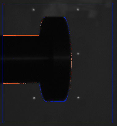
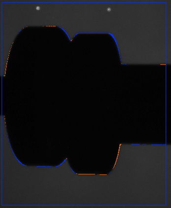
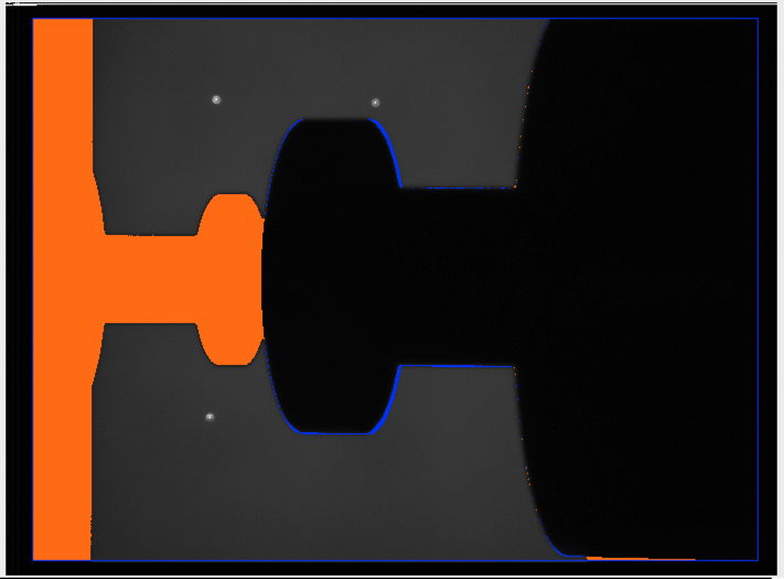
[15-DEC-23] We enhance our CPMS Manager 1.9 so that we can define analysis boundaries with the mouse, thus removing from analysis mounting components that we do not describe in our body models. By this means, the disagreement can in principle be zero, so its value, and a visual inspection of the colored pixels in the image, give us a measure of the quality of the fit. See CPMS_Manager_1V9 for appearance of the tool. We can now model only the flange and the first pipe. The larger base cylinders are out of view. We define the small and large flanges as separate bodies and fit both. We find that we must include in our small flange model the 0.5-mm, 45° chamfer on one face, or else the model is too wide for the silhouette.
22 16 416 0 0 0 # nominal large flange xyz and orientation
shaft 0 0 0 -1 0 0 # large flange shaft object, xyz and axis
33.78 0.0 33.78 7.24 19.0 7.24 19.0 29.39 # large flange, first pipe
29 18 416 0 0 0 # nominal small flange xyz and orientation
shaft 0 0 0 1 0 0 # small flange shaft object, xyz and axis
18.64 0.0 18.64 2.5 17.64 3.00 9.64 3.00 9.64 21.31 # small flange, chamfer, first pipe
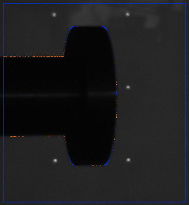
After fitting both flanges, our CPMS Manager display of one of the silhouettes looks as below. Note that the blue analysis boundaries have been brought in so they enclose the flanges and first pipes, but not the base cylinders.
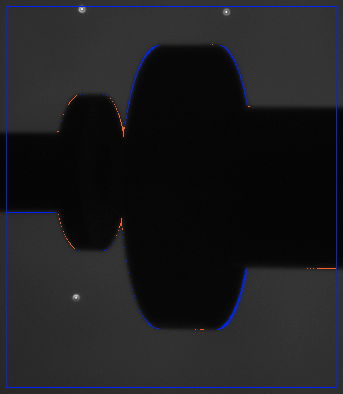
We displace the flanges ten times and fit ten times to obtain precision of the fit. We are not adjusting the rotation of the flanges about their axis of symmetry, but we are rotating them about the other two axes. We are using num_lines = 1000, threshold = "10 %", line_width = 1.
We drop the threshold from "10 %" to "5 %" and fit a few times. Our disagreement rises from ≈2000 pix to ≈4000 pix. We resolve to measure the disagreement as a function of threshold for the same pair of images. We save S1702660802_L.gif and S1702660802_R.gif. We increase threshold, displace our model, and fit for each value 5 to 20.
We select "13 %" as a robust threshold, tolerant of small changes in backlight intensity, and providing a near-minimum disagreement. During our work, we observe the fitter converging several times upon local disagreement minima for which the rotation of the flanges about the y-axis is opposite to the correct rotation. We arrive at these minima less often when we reduce the orientation scaling from 0.05 to 0.02.
We repeat our analysis of thirteen images of the small and large flange, this time fitting both flanges and using analysis boundaries that exclude the base cylinders. In the three data sets the large flange moves 6 mm in 0.5-mm steps first in the x-direction, then the y-direction, and finally in the z-direction.
Residuals in direction of motion over six millimeters are 11, 15, and 70 μm rms in x, y, and z respectively. The small flange does not move in any of these translations. The standard deviation of its position in any one of the movements is around 30 μm in x and y and 140 μm in z. We note that the small flange is half the diameter and our precision is twice as large.
We place our two flanges in the field of view of our CPMS. With our CMM we measure the face of the cylindrical base of each flange. We measure the axis of the pipe. We intersect the two to obtain the center of the base. We record the center coordinates and diameter of the pipe. In future, we will use the base center and axis to obtain the center of the face of the flange, which is what our CPMS is measuring. We measure the pose of both flanges with the CPMS, using recorded images.
We are translating the large flange in three dimensions between our five measurements. We are rotating the small flange about y. The axes of both flanges are horizontal. We expect the y-coordinate of the CPMS to agree with that of the CMM for both flanges. We expect the z-coordinate of the CPMS to agree with that of the CMM for the large flange. From these five points, it appears that our CPMS measures the y-coordinate of both flanges with an average error of +100 μm and standard deviation 30 μm. In z the average is 100 μm with standard deviation 125 μm.
[18-DEC-23] The new CPMS Manager 1.9 allows us to select our analysis bounds in both the left and right camera images before fitting. Thus we can ignore the mounting brackets or base cylinders. We select by control-clicking on the image and moving the mouse to the opposite corner of our desired bounds, then releasing the mouse.
We glue an 8-mm long, 2-mm diameter pin to the outer surface of one of our flanges. The pin is as close to radial as we can make it. Its center is 3.7 mm from the top face of the flange.
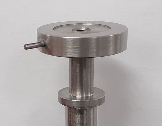
We use the following dual-object body model to describe the flange and its pin for the CPMS Manager.
26 38 463 0 0 0 # Pose of flange with pin.
shaft 0 0 0 0 -1 0 33.78 0.0 33.78 7.24 9.52 7.24 9.52 25.55 # Flange
shaft 16.89 -3.7 0 1 0 0 2 0 2 8 # Pin
With this model, we measure the pose of the pin and flange. We begin with the pin visible only in the right SCAM. Data 231218A. We move 12° in 1° steps. Our slope is 14 mrad/deg and residuals are 14 mrad. The ideal slope would be 1 deg/deg = 17.45 mrad/deg. We repeat in an orientation in which we can see the pin in both SCAMs. Data 231218B.
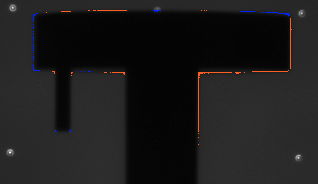
We move eight degrees, taking nine pairs of images. Our slope is 17.1 mrad/deg and our residuals are 3 mrad. We remove our radial pin and attach an axial pin to the back face of our small flange at radius 13.1 mm.
An axial pin can be mounted in one of the bolt holes that needs to be aligned. When the time comes to remove the pin, the two flanges will be flush, so the risk of contaminating the interior is reduced. We use the following model to represent the flange, pipe, and pin.
26 38 463 0 0 0 # Pose of flange with pin.
shaft 0 0 0 0 -1 0 33.78 0.0 33.78 7.24 9.52 7.24 9.52 25.55 # Flange
shaft 13.2 -7.4 0 0 -1 0 2 0 2 8 # Pin
With this model, we fit the rotation and position of the flange with its pin. We are using scaling "1 1 5 0.2 0.2 0.2", threshold "13 %", exposure 40 ms, and num_lines = 1000.
In our first movement of the axial pin, we start the pin at its leftmost position in the field of view of the CPMS. We move 13° in 1° steps. Data 231218C. We obtain slope 16.1 mrad/deg and residuals 12 mrad. We rotate the pin by 45° so that its movement across the field of view of the SCAMs is more pronounced as it rotates. Data 231219A.
Our axial pin gives us a rotation measurement with slope 17.52 mrad/deg and residual 8 mrad. Our precision in measuring rotation is better than 10 mrad rms. At a radius of 13.2 mm, our precision in locating a bolt hole in which we have placed a pin will be better than 130 μm rms.
[27-DEC-23] We mount our small and large flanges together, but this time we have the flanges facing one another as they should be, instead of having the small one with its narrow end facing the larger flange. We model the two flanges with the following CPMS Manager bodies.
{20 16 416 0 0 0 shaft 0 0 0 -1 0 0 33.78 0.0 33.78 7.24 19.0 7.24 19.0 30.0}
{25 15 416 0 0 0 shaft 0 0 0 1 0 0 33.78 0.0 33.78 7.24 9.64 7.24 9.64 30.0}
We measure the position of each flange with our CMM by intersecting the axis of the pipe with the outer face of the flange. We record the axis unit vector and the intersection. We record images.
For each pair of images, we define analysis bounds that include only our two bodies. In some cases, our images are overlapping. In others, the left flange pipe disappears into the left mounting bracket silhouette. We move the right flange a significant distance in x, y, and z between our several measurements, and we rotate the left flange by of order ±10°. In order to get our fit to converge, we sometimes have to move our model closer to the correct position manually.
We move the outer face of the flange as measured by the CMM to the inner face using the pipe axis vector. We compare with the CPMS measurement of the inner face center. In four of the six positions, we have x, y, and z agreeing for both flange centers within a fraction of a millimeter. But the other two positions have a 4-mm disagreement in x. Looking at the images, it appears that our CMM measurements are wrong for these two positions. We resolve to repeat, but keeping the left flange rotated very little with respect to the first, and being strict about measuring the back face of the flange.
[12-JAN-24] We have our two flange silhouettes overlapping. They are 1 mm apart and aligned in y and z. Only an x-translation of 1 mm is required to bring the two into contact.
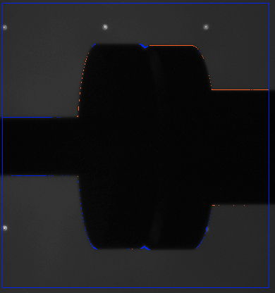
With the flanges overlapping, our resolution in z degrades.
[15-JAN-24] We add the base cylinder to our model of the large flange.
{20.305 15.820 412.945 0.000 0.012 0.009
  shaft 0 0 0 -1 0 0
  33.78 0.0 33.78 7.24 19.0 7.24 19.0 29.39 58.72 29.39 58.72 50.0}
{22.143 16.025 412.939 0.000 0.008 0.006
  shaft 0 0 0 1 0 0
  33.78 0.0 33.78 7.24 9.64 7.24 9.64 30.0}
The base of the small shaft is overlapped by the vertical, rectangular plate to which we fasten the flange, so we are unable to provide the same base cylinder object for the small flange.
Our resolution x, y, and z have improved dramatically with the addition of the base cylinder.
[19-JAN-24] We attach a pin to each of our two flanges. The pins are 2-mm diameter, 8-mm long precision pins with chamfered ends. We attach them with cyanoacrylate and measure their locations with calipers.
Our model of the two pins and flanges is below. This model includes the chamfers on the flanges, which are 10 mils on both sides.
{17.844 15.763 414.248 -0.149 -0.001 0.007
shaft 0 0 0 -1 0 0
33.27 0 33.78 0.25 33.78 6.99 33.27 7.24 19 7.24 19 29.39 57.71 29.34 58.72 29.9 58.72 51.1 57.71 51.61
shaft 0 13.24 0 -1 0 0
2 7.24 2 15.24}
{22.045 16.691 413.230 0.117 -0.021 0.009
shaft 0 0 0 1 0 0
33.27 0 33.78 0.25 33.78 6.99 33.27 7.24 9.53 7.24 9.53 25.55 18.64 26.05 18.64 28.05 17.63 28.55
shaft 0 11.79 0 1 0 0
2 7.24 2 15.24}
With the flanges overlapping in the CPMS view, the perimeter of a single pin is equal to the exposed perimeter of each flange, so the addition of the pins amplifies disagreement when the model is wrong, making the fit more sensitive.
[23-JAN-24] We position our large flange so that its center is at approximately the same y and z coordinates as the small flange. We separate it by roughly 9.5 mm in x and move the large flange towards the small flange with our x-direction stage. At each position, we measure the separation of the flanges with our calipers and with the CPMS using our two-pin model with flanges.
When we subtract a straight line fit we get the following for the CPMS measurements.
[24-JAN-24] We place our large flange roughly 0.5 mm away from the small flange in the x-direction and adjust in y and z until our CMM says that they are within 50 μm of one another in these coordinates. We move the large flange upwards in y by 2-mm with our vertical stage (forward movement), and then downwards again (backwards). At each position we measure the separation of the flanges in the y-direction with the CPMS. We fit a straight line and obtain an intercept that is within 50 μm of zero for both the forward and backward series of points.
In the residuals we note symmetric outliers for forwards and backwards at 800 and 850 μm.
[30-JAN-24] We repeat our experiment of 24JAN24, but we move in z from our starting position instead of in y. We fit a straight line and find the intercept is within ±100 μm.
[31-JAN-24] We place the large flange in ten randomly-generated separations 0 mm ≤ x ≤ 2 mm, −1 mm ≤ y ≤ 1 mm, and −1 mm ≤ z ≤ 1 mm. We lose the pair of images associated with the first position. We reject the final position because the flanges are touching and not exactly parallel, so we suspect the flanges have rotated. We use the remaining eight to study the stability of the fit. We set our threshold to "16 %", num_lines to 1000, line_width 1. The correct x-orientation of the large flange is roughly -190 mrad, which we confirm by eye. When analyzing a significantly new position, the fitter can converge to an x-orientation of +190 mrad and there find a minimum in disagreement that is 125% of the correct minimum, but leads to an error in x-position of about 0.5 mm.
For the eight useful positions, our precision in measuring separation is 46 μm in x, 53 μm in y, and 330 μm in z. Our average measurement of separation is consistent with zero in all three coordinates. The small flange does not move, and the standard deviation of its position is 58 μm, 13 μm, and 180 μm in x, y, and z respectively.
[05-FEB-24] It takes roughly forty seconds to analyze one set of stereo images of our two flanges with pins on a new Windows laptop. If we reduce the number of lines in our tracing, the fit loses its accuracy. Our modelled body fill routine is inefficient. The CPMS accuracy is dominated by convergeance of the fit. In our 50-cm system, with backlights at 100 cm, the accuracy in measuring separation with a single fit is 50 μm in x and y, and 300 μm in z. Our average error over ten fits to ten random positions is 0 μm in x, 25 μm in y, and 90 μm in z.