Technical Proposal for Subcutaneous Transmitter
© 2004, Kevan Hashemi,
Open Source Instruments Inc.
Contents
Introduction
The DSI Transmitter
How Antennas Work
The OSI Transmitter
Feasability Studies
Draft Transmitter Design
Draft Receiver Design
Data Acquisition Hardware and Software
Target and Minimum Performance
Remaining Challenges
Development Schedule
Other Devices
Conclusion
Introduction
We propose to develop and build Subcutaneous Transmitters in collaboration with Dr. Walker at the Institute of Neurology. The institute will pay OSI a fixed sum for materials, development, and delivery of prototypes. The institute will develop suitable packaging for the transmitters, inform us of the details of practical applications, test the transmitters in live animals, and determine if their measurements are accurate enough and fast enough. After development, we will deliver enough hardware to allow Dr. Walker to run a three-month experiment on half a dozen animals. We expect each receiver to receive data simultaneously from dozens of animals within a five-meter radius. The animals might live together in a large cage, or in separate cages. The receiver will operate with our stand-alone data acquisition hardware. Laboratory computers running our LWDAQ software will acquire transmitter data over the local area network. We will extend our existing data acquisition software to support data acquisition from the transmitters, and we will provide a convenient interface to Dr. Walker's existing analysis software.
The DSI Transmitter
Although we do not have the circuit diagram of a DSI transmitter, we are confident that we understand approximately how it works. It transmits information by means of a coil of wire through which it allows a capacitor to discharge suddenly, as shown in Figure 1. The current passing through the coil builds up a magnetic field. Ignoring any resistance in the coil, all the energy from the capacitor is transferred to the magnetic field. When the capacitor is empty, the magnetic field energy dissipates suddenly through a diode.
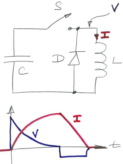
Figure 1: Magnetic Pulse Generation. At t=0 the capacitor is full, there is no current in the coil, and the switch closes. The voltage across the coil drops to zero and then jumps down to one diode drop below zero while the energy of the magnetic field dissipates as heat in the diode.
If we place another coil nearby, the magnetic field generated by the transmitter coil will pass through this second coil. As the magnetic field in the tranmsitter coil builds up and collapses, it will induce an electro-motive force (EMF) in the second coil in accordance with Faraday's Law. The receiver measures this EMF and so receives the pulse. The amplitude of this pulse is strongly dependent upon the location of the transmitter, and cannot be relied upon to convey information. But the time at which the pulse arrives, if the pulse is short enough, can be compared to the time at which a second pulse arrives, and this difference in time can be used to convey information.
Consider what happens to the energy stored in the capacitor when there is no receiver coil nearby. The energy moves from the electric field between the capacitor plates and into the magnetic field surrounding the coil. It withdraws from the magnetic field and dissipates as heat in the diode. If we imagine a large enough volume around the transmitter, we see that the energy outside this volume is negligible. Energy is not propagating out into space. It is dissipating in the diode as heat. The transmitter merely stores energy temporarily in its immediate vicinity, takes it back again, and dumps it into a diode.
In the end, the energy that was stored in the capacitor does indeed spread out into space, but it does so as heat, and carries no information useful to us.
At ranges greater than a few centimeters, the magnetic field around the transmitter coil is fully developed. Consider how the strength of the field decreases with range. Suppose the magnetic field strength (measured in Tesla) decreased as the inverse of the range. The energy density per unit volume would be proportional to the square of the field strength. With the field decreasing as the inverse of the range, the energy density would decrease as the inverse square of the range. But if we integrate this energy density from range ten centimeters to infinity, we see that the total energy of the field is infinite, and extends through the entire universe. We already know that this cannot be the case, because the pulsed magnetic field establishes itself in finite time, and collapses in finite time, leaving no energy unaccounted for in space. The field strength must decrease more quickly than the inverse of the range. Electro-magnetic field equations do not yield non-integer powers of range, so the field strength must drop at least as fast as the inverse square of the range, which means the energy density of the field must drop at least as fast as the inverse fourth power of the range.
If, on the other hand, the transmitter were to propagate energy outwards into space as radio waves, conservation of energy would dictate that the propagating field strength decrease only as the inverse of the range. But the DSI transmitter does not transmit energy into space.
Compared to a radio transmitter, the pulse transmitter's range is severely limited by the rapid decrease in its magnetic field strength with range. The energy available at the receiver decreases as the inverse fourth power of the range, as compared to the inverse second power we would get from a radio transmitter. The pulse transmitter uses most of its power allowance creating the largest possible magnetic pulses so that it can operate at the greatest possible range. Even with its battery power dedicated to pulse generation, the pulse transmitter's range is measured in tens of centimeters.
In short: the fundamental weakness of the DSI design is that it burns its battery power in a diode instead of propagating it out into space. Because most of the battery power is consumed by the act of transmission, very little is left for measurement accuracy or communication logic.
How Antennas Work
In order to make it clear why it is possible to build a miniature transmitter with operating range over ten times greater than that of the DSI transmitter, we now embark upon a qualitative analysis of radio transmission and reception.
Imagine an electron sitting alone in a vacuum, and an electric field sensor at a point some range from the electron. The electric field strength we measure decreases as the inverse of range, and the total energy of the field around the electron is infinite. If we move the electron a short distance, its infinite field must change accordingly. But the field cannot change immediately at all ranges. Maxwell's field equations dictate that changes in the electric field propagate outwards at a speed equal to the inverse square root of the product of the permability and permittivity of a vacuum (See Figure 2).
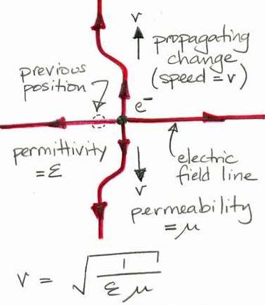
Figure 2: Propagating Disturbance in an Electric Field. The electron recently moved to the right.
When we look at Maxwells equations, we find that it takes energy to move an electron. We must exert a force upon it. The work we do when we move the electron goes into forcing the field around the electron to change, and this change must propagate outwards to infinity if the entire field around the electron is to adjust itself to match the electron's new position. At any point in time, the energy we put into moving the electron exists at the propagating kink in the field lines. In a vacuum, this kink propagates at three hundred million meters per second.
Imagine a second electron in the path of the propagating kink of Figure 2. As the kink passes over the electron, the electron experiences a force to the left. We move the first electron to the right, and the second electron experiences a force to the left some time later. The magnitude of the force is proportional to the local field strength, which we have already concluded to be proportional to the inverse of the range. The time delay between the movement of the original electron and the occurance of the force on the second electron is equal to the range divided by the speed of light.
Aside: How can we say that it is the first electron that moved and not the second one? Surely we could pick a frame of reference on the first electron, and consider the second electron to be the one that is moving. The first electron would experience a force some time later, not the second electron. But we can prove that it is, in fact, the second electron that experiences the force some time later, not the first. So what is wrong with choosing the second frame of reference?
If we move an electron at a constant velocity from left to right, we find that the field around it takes on a static shape, and our second electron will experience exactly the same force as if it were the one that was moving at constant velocity, and the first electron were stationary. The kinks in the electrostatic field around an electron are not generated by its velocity, but instead by changes in its velocity. It is the acceleration of charges that takes work and causes the propagation of energy through space.
Let us suppose our two electrons are in two separate wires. With some kind of electrical contraption, we push the first electron to the right in the wire. The second electron will be pushed to the left in the second wire. We transmit energy from one wire to the other.
When it comes to pushing electrons, however, we are faced with some interesting technical difficulties. We move electrons along a wire by pushing extra electrons in at one end, and allowing electrons to come out the other end. The result is a net transfer of electrons from one place to another. But we must consider what happens to the electrons after they leave the wire. They go around through our power supply and come back to the other end of the wire. If we reverse the direction of the electrons in our wire, we also reverse the direction of the electrons in the rest of the circuit. We can think of a loop of wire with an alternating voltage source at one point in the loop, pushing electrons one way and then the other way around the loop (see the left side of Figure 3). When we look at the loop from a great enough distance, we see no net movement of electrons, only a circulation. This circulation creates a magnetic field that will exert a force upon an electron, but the strength of the magnetic field drops as the inverse fourth power of the range. We do not have transmission of power into space.
We appear to be a bit stuck.
Suppose we increase the frequency of our alternating current in the loop. At a high enough frequency, we encounter another electrical phenomenon, closely related to that of electromagnetic propagation through space, which turns out to make power transmission possible. If we push a bunch of electrons into the end of a wire, it takes a while for the effect of this concentration of electrons to propagate along the wire. The effect propagates at a certain speed, call it v. If we are alternately pushing and pulling electrons into and out of the end of the wire with frequency f then we will have waves propagating along our wire with length v/f. Figure 3 shows what happens when the circumference of our loop is equal to the wavelength of our alternating current.
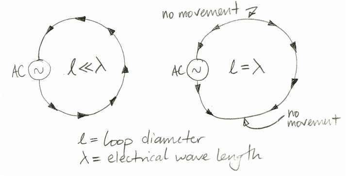
Figure 3: Electrons Moving Around in a Loop. At just the right frequency, there is perfect up-and-down, and left-to-right.
We find that we have a net downward movement of electrons at one point in time, and we will have net movement in all other directions at other times. An electron on the axis of the loop will experience a force of constant magnitude, in a direction that rotates about the loop axis. An electron off to one side of the loop will experience an alternating force. The loop radiates power in all directions, and is the closest we can come to an omnidirectional antenna. We call it a loop antenna.
When the circumference of a loop antenna is equal to the wavelength of our transmitting signal, we say it is tuned to our transmission frequency, or that the loop antenna is resonant at the transmission frequency. When we calculate the electrical energy required to force current through the loop, we find that all this energy is propagated into space. So, it turns out that we are rescued from the loop dilemma by the short wavelength of high-frequency signals, and we can build an efficient electromagnetic energy transmitter out of a loop of wire.
An alternative to the loop antenna is the dipole antenna, which we show in Figure 4. The dipole antenna is more directional than the loop antenna, because it transmits no energy in the direction parallel to the dipole wires. But it is an interesting antenna to consider, because the wires end in mid-air, and no electrons come out of the end, and yet we still do work pushing electrons into the base of each wire.
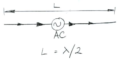
Figure 4: Dipole Antenna. Note that no electrons flow out of the end of the wires.
A quarter-wave antenna, as shown in Figure 5, is a dipole antenna on top of a ground plane.
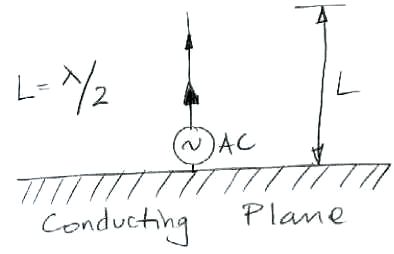
Figure 5: Quarter-Wave Antenna.
We used a cross between a dipole and a quarter-wave antenna successfully in our subcutaneous transmitter feasability studies.
The OSI Transmitter
While writing this technical proposal, we came to understand that a loop antenna should work very well in our subcutaneous transmitter. It is clear that a loop running around the edge of the transmitter circuit board is more convenient than a piece of wire sticking out of the circuit board. We used a quarter-wave antenna for our feasibility studies. A quarter-wave antenna is easier to tune han a loop. All you have to do is cut bits off the end of the quarter-wave antenna, while you have to cut and reshape a loop. But we will assume in the following paragraphs that our final subcutaneous transmitter will use a loop antenna around the edge of its circuit board.
Consider a tuned, square loop antenna. Its width and height are a quarter wavelength. In air, the speed of an electrical signal traveling around the loop will be roughly three hundred million meters per second. At a transmission frequency of 100 kHz, our loop would be 750 m wide. At 1 GHz, it would be 75 mm wide. We hope to build a subcutaneous transmitter 18 mm square and 7 mm high, so that its volume compares with that of the DSI mouse transmitter. A 75-mm wide loop antenna would be inconvenient.
But it so happens that the physical properties of animal bodies help us significantly here. The permittivity of water, which is most of what an animal body is made of, is eighty times that of air. Electrical signals traveling around a loop antenna immersed in water will travel nine times more slowly than in air, so the tuned loop antenna will be nine times smaller. One ninth of 75 mm is 8 mm. But our transmitter will probably be just beneath the skin of a rat, so it will be half in water and half out of water. So long as the wavelength is less than 18 mm, we will be able to fit a tuned loop antenna on our circuit board. We might find that a 12-mm loop works well enough for both for total immersion of the transmitter in a large animal body and just-under-skin immersion, or we might find that we need two different loops for these two applications.
The 900-MHz cordless phone has been replaced by the 2.4-GHz phone, and will soon be replaced by the 5-GHz phone. The 900-MHz wave band is for public use, is relatively free of regulation, is going out of fasion with cordless phones, and is served by a wide range of inexpensive and well-developed electronic components. We can build a compact 1-GHz transmitter from these parts, and build an efficient antenna on a small circuit board.
Feasability Studies
We designed some simple test circuits and layed out the Subcutaneous Transmitter Test Board (A3001). Figure 6 shows the circuit board. We obtain the circuits by cutting the board into four pieces. The four circuits are the Modulating Tranmsitter, the Downshifting Receiver, the Miniature Transmitter, and the Amplifying Demodulator.

Figure 6: Subcutaneous Transmitter Test Board (A3001) printed circuit board. The circuit board part number is A300101A.
We tested the Modulating Transmitter, Downshifting Receiver, and Miniature Transmitter. We presented our results in three separate and detailed reports. In the sections below you will find summaries of these reports, and links to the reports themselves.
Modulating Transmitter
Our first concern when considering the feasability of a battery-powered subcutaneous transmitter operating at one gigahertz is whether of not we can obtain efficient transmission with a simple low-power circuit. In theory, we can do so, but in practice, we can imagine encountering all kinds of technical difficulties. Radio transmission and antenna design are regarded as black arts in the electronics community. Cell phone manufacturers do not publicize their antenna designs. Nor do cordless phone designers. When we opened up an old 900-MHz phone and looked inside, the transmission and reception circuits were complicated, with PCB tracks used for delay lines in several places, and a large number of discrete components. Data transmission using a one gigahertz carrier is supported by several chip sets, but we imagined using a simple 1-GHz voltage controlled oscillator (VCO) to create the transmission signal and perform the modulation in one step.
We selected a low-power VCO from Maxim Semiconductor, the MAX2624. We called them and asked about using their chip as a transmitter and modulator combined, and they said it was not designed to be used that way. Despite these pessimistic assertions on the part of the manufacturer, we were able to transmit as much 1-GHz power as we had hoped, and modulate its frequency at 10 MHz, which is adequate for 20 MBits/s data transmission. Here is the complete Modulating Transmitter (A3001A) report, with description of the circuit components and calculations, and here is the circuit diagram.
Our study shows that we can transmit 1-GHz power with a simple quarter-wave antenna. We can obtain this power from tiny VCO chip that consumes only 8 mA. The chip will turn on and off in less than a microsecond. We can modulate the outgoing transmission frequency at 10 MHz, which is adequate for 20 MBits/s data rate. If we transmit a 10-bit synchronizing signal, a 20-bit identifier, a 16-bit data sample, and a 4-bit checksum, we will need only only five microseconds for the entire communication. We can do this four hundred times a second, for 400 SPS (samples per second) data rate, and our tranmission power consumption will be less than 20 μA. The battery we are considering is 18 mm in diameter and 3 mm high, and provides 120 mA-hr of current. Our current consumption budget during a three-month operating lifetime is around 50 μA.
Given that each transmitter in a laboratory will be transmitting for only 5 μs out of every 2.5 ms, we see that it is possible for many transmitters to share the same receiver, provided the receiver is within range. The checksum on each data transmission will allow the receiver to detect collisions between data transmissions and ignore corrupted data. Although we will miss out on samples every now and then, this will matter little because each sample will be time-stamped by the receiver and the data acquisition software will simply reconstruct the underlying 100-Hz signal despite the occasional missing sample.
In theory, our transmitter is powerful enough to operate over a 5-m range together with a dozen other transmitters, and share the same receiver.
Downshifting Receiver
Our next concern was the working range of our transmitter. We tested our Modulating Receiver, and again we met with success. Here is the complete Downshifting Receiver (A3001B) report, with description of the circuit components and calculations, and here is the circuit diagram. We concluded that in the absence of strong 900-MHz interference from cordless phones, we could operate a 20-MBit/s data link between our battery-powered transmitter and a receiver five meters away, and do so simultaneously with a dozen other transmitters.
Miniature Transmitter
Our next concern was the effect of the orientation of the transmitter upon the power we receive, and the effect of water upon the length of our quarter-wave antenna. Here is the complete Miniature Transmitter (A3001D) report with description of the circuit components and calculations, and here is the circuit diagram. We found that it is possible to reduce the received power dramatically with precisely the worst orientation of the transmitter, but that almost all orientations would supply adequate power to operate at a range of three meters, and probably five meters.
We also found that our quarter-wave antenna was only 17 mm long at the edge of a beaker or water, instead of 75 mm in air. We were able to transmit half as much power out of a beaker with a 17 mm antenna as we tranmsitted with a 75-mm antenna in air. We conclude that we will be able to transmit adequate power out of a rat, and that the wavelength of our 1-GHz transmission frequency will be closer to 70 mm under the skin of a rat, compared to 300 mm in air.
Other Tests
We knew that we would need a 40-MHz clock to drive our data transmission. We build a 40-MHz ring oscillator in a programmable logic chip similar to the one we propose for the transmitter. This oscillator can be turned on and off in a matter of nanoseconds. When it runs, it consumes less than 4 mA, which is less than any other 40-MHz oscillator we could find. The ring oscillator has the added advantage that it occupies no additional board area, because it is contained within the logic chip.
We tried to build a low-frequency oscillator with the inputs and outputs of a logic chip, and a resistor-capacitor (RC) network, but the slow transition of the RC divider voltage through the chip's input logic threshold caused oscillations and feedback in the logic circuit. We will use a separate micro-power low-frequency oscillator instead.
Draft Transmitter Design
Figure 7 is a block diagram of our proposed Subcutaneous Transmitter. The diagram names the critical low-power integrated circuits upon which the entire design depends. A year ago, the zero-power programmable logic chip in a 6-mm square ball grid array package was not available. The low-power 1-GHz oscillator is another new part. It seems to us that it would have been impossible to meet our specification without parts that have become available in the past year.

Figure 7: Schematic of the Subcutaneous Transmitter. The entire circuit runs of a 3-V Lithium battery, but we need a 1.8-V regulator to provide internal power to the logic chip. We disconnect the battery from the circuit by putting a magnet outside the circuit's magnetic reed switch.
The input to the transmitter is two wires from a probe of some sort. We will decide the exact form of these leads in consultation with Dr. Walker. We do not see the choice of leads, or the exact impedance seen by the probe, as a source of difficulty.
We use a dual micro-power op-amp from National Semiconductor, the LMC6442 to build an instrumentation amplifier to receive the probe signal, and a low-pass filter to remove frequencies above 100 Hz, in preparation for 400-Hz sampling. The total quiescent current of these input circuits will be less than 8 μA.
We digitize the amplified and filtered input with a low-power sixteen-bit serial-output analog-to-digital (ADC) converter, the LTC1864 from Linear Technology. At a sample rate of 400 Hz, the LTC1864's automatic shut-down circuits ensure that it consumes less than 10 μA.
At the heart of our circuit is an in-system programmable (ISP) logic chip from Lattice Semicondutor, the ispMach4064Z-37M56C. This amazing new chip consumes 10 μA quiescent from a 1.8-V supply, and comes in a 6-mm square 56-ball grid array package. We have never used a ball grid array package, and doing so is one of the technical problems we must overcome in our printed circuit board layout. But the problem has obviously been solved by many people, and we have no doubt that we can solve it also. The ISP chip obtains samples form the ADC 400 times a second, turns on the transmitter, and sends out the stream of bits that make up each data transmission. The ISP chip is in-system programmable, which means you can configure its 64 or 128 logic macrocells in any way you want simply by applying power to the chip and connecting its programming pins to the Lattice Semiconductor programming cable.
If we are to transmit a stream of bits at 20 MBits/s four hundred times a second, we need clock signals to control our logic circuits. We will use the OV1564C2 from Gollege as our low-frequency oscillator. This part consumes at most 2 μA, and provides a 32-kHz clock signal. Our logic chips will divide down the 32-kHz to produce 400 Hz timing. During data transmission, we will turn on a 40-MHz ring oscillator inside the logic chip. The frequency of this oscillator will not be precise. We estimate that the transmission bit rate will vary by ±25% from one transmitter to the next. But we will design the receiver to deal with the variable bit rates. The ring oscillator will consume about 4 mA during the 4-μs data transmission. We will allow another 1 mA for a counter that counts the data bit number within the transmission. The transmission logic should consume about 5 mA during transmission.
The logic chip requires 1.8 V to run its zero-power internal circuits. We will use the MAX1726 micro-power regulator to create 1.8 V from our 3-V battery supply. This regulator has a quiescent current of 2 μA.
We have already discussed the MAX2624 voltage-controlled oscillator. This part consumes 8 mA while active. When combined with our transmission logic current consumption, we see the total transmission-time current consumption should be less than 13 mA. If we transmit for 4 μs every 2.5 ms, our average transmission consumption is less than 20 μA.
The final part of our transmitter is a magnetic reed switch that allows us to disconnect the battery from the circuit by placing a magnet against the switch, outside whatever coating we have placed around the transmitter.
When we add up our total average current consumption we get 8 μA for the input amplifiers and filters, 10 μA for the ADC, 10 μA for the logic chip when it is not transmitting, 20 μA for transmission activity, 2 μA for the regulator, and 2 μA for the low-frequency oscillator. That's a total of 52 μA. With a 120-mA-hr battery, we expect 100 days of continuous operation.
With current consumption under control, we are now concerned with the space consumed by the parts. Figure 8 shows the battery on top of the board, and a side view showing the depth of the transmitter, and the low-profile parts on the bottom.
Figure 8: Sketch of the Top of the Subcutaneous Transmitter.
Figure 9 shows the bottom of the board, with shapes giving the approximate size of the integrated circuits.
Figure 9: Sketch of the Bottom of the Subcutaneous Transmitter. The "PLD" is the in-system programmable(ISP) logic chip.
For resistors and capacitors, we will use the tiny 0402 package, which is 1 mm long, 0.5 mm wide, and 0.35 mm high. We will be able to place such parts beneath the battery on the top side if we have to. The design of the battery's legs causes it to sit up off the board by 0.5 mm.
We are confident that we can fit all necessary parts on an 18-mm square circuit board, and take up a total depth of only 7 mm. This will make the total volume of the transmitter less than 2 ml. Its weight will be roughly 3 g. Its operating life should be at least three months.
Draft Receiver Design
The receiver will use a commercially-made 900-MHz antenna, such as the HG908U to present a large effective aperture to transmitters at the same height above the laboratory floor. The incoming signal will be amplified and demodulated and converted into a logic level. This level will be zero at all times except during the reception of an SCT data burst. The data burst begins with a sequence of bits that allow the receiver logic to lock onto the frequency of the subcutaneous transmitter's clock, and then identify the first bit of the tranmsitter's identification number. After the identification number will come the sixteen-bit sample, and a checksum. If the checksum matches the identification and sample, the receiver stores the two numbers together with a time stamp (accurate to the millisecond) as a data entry in its RAM (random access memory). The total space taken by each data entry will be about ten bytes.
The receiver is a LWDAQ (Long-Wire Data Acquisition) Device. We do not yet have a one-page introduction to our LWDAQ electronics, so we will have to point you to the specification. A LWDAQ Device connects to a LWDAQ system through its RJ-45 socket and a LWDAQ cable. You can use standard straight-through Ethernet cables, or make your own LWDAQ Cables, as described in the Cable-Making Manual. If you make your own cables, they can be up to 130 m long, so you will have no problem running them around your lab to the driver from your receiver or receivers.
The SCT Receiver will allow the LWDAQ system apparently simultaneous access to its memory, to transfer acquired data to the LWDAQ's main memory on its LWDAQ Driver (see below). The LWDAQ must retrieve data fast enough to avoid the receiver over-writing old data with new data. The receiver will transfer data at up to 400 kBytes/s. Each transmitter creates 400 entries per second, or 4 kByte/s.
When two transmitters send a data burst at the same time, the receiver will recognise a burst collision and discard both samples. A random timing disturbance in the transmitters will ensure that the probability of more than two consecutive burst collisions is negligible. The transmitted signal bandwidth will almost always keep up with the 100-Hz bandwidth of the transmitter's input filter.
If we find that we need two receivers to accommodate the range of orientations of the transmitters in a laboratory, both will operate simultaneously, and the data acquisition system will synchronise their clocks so that their time stamps can be used to eliminate duplicate data entries.
Data Acquisition Hardware and Software
In addition to SCTs and SCT Receivers, we will provide Dr. Walker with all hardware and software necessary to deliver the transmitter data to his analysis software.
The SCT Receivers will connect to a LWDAQ Driver with Ethernet Interface (A2037E). The A2037E is a textbook-sized black box with an RJ-45 Ethernet socket on one side and eight LWDAQ Driver Sockets on the other side. You plug the driver into a 10-Base-T Ethernet, and run our LWDAQ Software on your data acquisition computer, somewhere else on the Internet, or on the same Ethernet. Our software is free, and runs on Linux, OSX, and Windows. The data acquisition computer communicates with the driver over TCP/IP. We will create a new SCT (subcutaneous transmitter) instrument for the LWDAQ program's Instrument menu. This instrument will acquire data from a receiver and save it to disk or transfer it to another data acquisition program on the same or another computer over TCP/IP.
The data rate out of a LWDAQ Driver (A2037) is limited by the embedded computer on the driver that runs its TCP/IP stack. This computer is the RCM2200 from Rabbit Semiconductor. It transmits up to 160 kBytes/s. Each SCT data sample takes up roughly ten bytes. Each SCT transmits 400 SPS, so each requires a data bandwidth of 4 kBytes/s. The driver must also transfer data from the SCT Receiver, and this it does at 400 kBytes per second (two byts at a time in 4-μs serial tranmsissions). We might also be limited by the data rate across the local Ethernet, but if this data rate is a problem, we can always connect our data acquisition computer directly to the A2037E, and obtain the maximum 160 kBytes/s. Even if we were acquiring data from an airport wireless network, we can expect a data rate of over 20 kBytes/s, so we would be able to acquire data continuously from five SCTs at a time half way around the world.
In a laboratory with a local ethernet, we can expect any computer on the network to acquire data continuously from at least a dozen transmitters, and probably thirty.
Here we give our target performance specification and our minimum performance specification. We are almost certain of our ability to meet the minimum performance, and confident that we will meet the target performance. If the target and minimum specification differ, we give the minimum in parenthesis.
- Length 18 mm
- Width 16 mm
- Height 7 mm
- Volume 2 ml
- Weight 3 g
- Battery 3-V 120 mA-hr Li
- Input Impedance: 10 MOhm differential
- Input Dynamic Range: ±10 mV or ±100 mV
- Input Bandwidth: 100 Hz
- Input Gain Accuracy: ±1%
- Input Linearity: ±0.1%
- Data Transmission Rate: 400 samples per second
- Data Format: 16-bit digital with 24-bit ID (16-bit digital with no ID)
- Range: 3 m (30 cm)
- Shelf Life: over 1 year (1 year)
- Operating Life: over 4 months (2 months)
- Transmitters per Receiver: 10 (1)
- Disable: by applying a magnet
- Transmitter cost each, uncoated, no sensor wires: $200 US
- Receiver cost each, with antenna: $2000
- Total cost per animal: $400 ($500)
We see that the cost per rat is strongly a function of our success in meeting our target range specification and our target number of transmitters accommodated by each receiver. If we meet our target, the receiver cost will be $200 US. If we miss out target badly, we will need to install a receiver under each cage. But this receiver will be simpler than the one we would use to receiver signals from ten rats at once, so it will cost less. Hence our per-animal cost does not rise to higher than $500 in the list above.
Remaining Challenges
Here are the greatest remaining technical challenges in our development of the Subcutaneous Transmitter. Each will take work, and some will require hours of thought, but we are confident of success in each case.
- 56-pin BGA (Ball Grid Array) mounting and footprint required by logic chip
- Random disturbance of sampling period to avoid burst collisions between precise oscillators
- Snap-off side panel on PCB to allow programming of logic chip during assembly
- Cordless phone interference
- Transmission wavelength in live rat
- Loop or dipole antenna in live rat
- Working range with live rat in all orientations
- Sterile coating and wire connections
- Array antenna for receiver
- Phase locking in receiver to recover transmitter data
- Burst collision recognition in receiver
Development Schedule
As we layed out in our original quotation, OSI commits to the following development schedule and payment plan.
Technical Proposal
We submit this technical proposal, plus a sample Miniature Transmitter with a few spare batteries, and a sample Downshifting Receiver, for Dr. Walker to test. We will invoice The Institute of Neurology for £3,000 for our development efforts so far, and use this money to pay for the materials required for the next state of development.
Dummy Transmission Circuits
Within eight weeks of receiving payment for our Technical Proposal, we will build a Miniature Transmitter with a logic chip on board and an oscillator. This device will transmit a data burst every 2.5 ms. Instead of a sixteen-bit ADC sample, the data burst will contain the output of a sixteen-bit counter. We will build five of these and send three to London for testing. We will build a Receiver circuit that reproduces the data bursts at its output. We will be able to see the bits of the data burst on an oscilloscope. We will build four of these receivers and send two to London. The purpose of these circuits will be to allow Dr. Walker to determine the effective range of the transmitters in live rats, and to try out their ideas for sterile coatings for the circuit. An integral part of the tests will be trying out different antenna types and lengths. Our hope is that a loop antenna wrapped around the border of the transmitter circuit will suffice, so that we will not have to deal with a protruding straight wire from the transmitter.
Kevan Hashemi, of OSI, will visit The Institute of Neurology to assist with the tests. The cost of this trip is included in the cost of this stage of development.
After delivery of the circuits, we will invoice The Institute of Neurology for £5,000.
Data Transmission and Reception Circuits
Within eight weeks of receiving payment for our Dummy Transmission circuits, we will build fully-functional transmitters with analog input amplifiers and ADCs. We will send four to London. We will build fully-funcitonal receivers, and add a new SCT instrument to our LWDAQ software. We will send two receivers to London, along with a LWDAQ Driver and cables. Dr. Walker will connect animal body signals to the transmitter analog inputs, and these will be digitized and transmitted to the receiver from four rats simultaneously. The LWDAQ program will run on a computer in the lab, connected directly to the LWDAQ Driver, and record the transmissions from all four rats. We will set up a connection between the LWDAQ program and Dr. Walker's data analysis and plotting software.
Kevan Hashemi, of OSI, will visit The Institute of Neurology to assist with the tests. The cost of this trip is included in the cost of this stage of development.
After delivery of the circuits, we will invoice The Institute of Neurology for £5,000.
Prototype Circuits
We will discuss the results of all tests we have performed so far with Dr. Walker, and agree upon the specification and particulars of the prototype circuit designs. We deliver 10 transmitters, 2 receivers, 1 additional LWDAQ driver, 20 additional cables, an imporoved version of the LWDAQ software, and documentation describing all circuits and software, within twelve weeks of receiving payment for our Data Transmission and Reception circuits.
Dr. Walker will then take several months to test the new devices in an experiment of some sort. After that, they are free to write a paper describing their results. All our documentation and circuits will be available on the OSI website for them to refer to in their work.
After delivery of the circuits, we will invoice The Institute of Neurology for the final £7,000 of the SCT development purchase order.
Other Devices
Because the SCT system uses the existing LWDAQ hardware and software, it will be easy for users to add high-resolution cameras, thermometers, and other sensors to the system, and synchronize their operation with data taken from the transmitters. The frame rate from the high-resolution cameras is, however, only one or two frames a second, limited by the data transmission speed of our existing TCP/IP communication hardware. But we could implemet a low-resolution camera operating at five frames per second, which might be fast enough to record the behavior of animals during interesting activity detected by the SCTs. In the long run, we will be designing at OSI a faster TCP/IP connection, which will provide high-resolution images at five frames per second, and low-resolution images at twenty frames per second.
Conclusion
We are confident that we can provide Dr. Walker with ten subcutaneous transmitters equal to or superior to those manufactured by DSI. We can do so in thirty weeks, and at total cost of £20,000. This cost is comparable to the total cost of equipping the same laboratory with the same number of transmitters from DSI. Subsequently, we will be able to supply transmitters and data acquision hardware at a far lower cost than that charged by DSI. Our software will be free.
We expect that the transmitters we build will be able to share receivers, and operate at over ranges up to 5 m. At the end of his experiments, Dr. Walker will be able to write a paper presenting his results, and he will be able to point his readers to our Open Source Instruments website, where they will find circuit diagrams, printed circuit board layouts, user manuals, and detailed descriptions of the operation of each circuit used in his experiments. All the work done at OSI will be distributed to the public for free. In addition, his readers will be able to purchase the same hardware from OSI directly.