Note: This document was previously entitled "Seizure Detection".
[05-AUG-22] The Event Classifier in the Neuroplayer Tool provides automatic detection of a wide variety of events in local field potential (LFP) and electroencephalograph (EEG) recordings. It operates upon signals recorded by subcutaneous transmitters (SCTs) from live, freely-moving laboratory animals. Other programs that run in the LWDAQ Software environment perform data export, power band analysis, and event consolidation. Our objective is to detect rare events in continuous recordings. We may count these events, measure their duration, or respond to them with a real-time stimulus delivered to the subject animal. We may have two thousand hours of EEG from a dozen animals and we want to count inter-ictal spikes that occur roughly once per hour. We want to count spikes with a precision of ±0.1 per hour, which means our detection algorithm must generate no more than one false positive per ten hours. The probability of a false positive in any one interval must be of order 0.001%. In order to achieve such a los false positive rate, the EEG recording must be free of movement artifact, devoid of electrical noise, and uninterrupted by wireless reception failure. The success of the event detection algorithms is founded upon the high fidelity of the recordings we obtain from our SCTs. We describe our latest event-detection metrics in Event Classification with ECP20. Most user of our Subcutaneous Transmitter (SCT) system use the Event Classifier to analyze their data, as well as some users of other telemetry systems, who translate their recordings into our NDF format so that they can make use of our Event Classifier [1, 2, 3]
Reception of wireless messages from a moving animal cannot be 100% reliable, but it can come close. Before you begin a study, we recommend you ensure that your telemetry system is set up correctly and reception from freely-moving animals is at least 98%. Pick the best electrode, and establish a procedure for securing the electrodes in place to avoid movement artifact. We discuss our choice of electrodes in Electrodes. We present our own understanding of the sources of EEG in The Source of EEG. For example recordings, see Example Recordings.
[19-JUN-18] By baseline signal we mean an interval of EEG that does not contain any unusual event. This definition is vague, and proves to be difficult to define in the logic of seizure detection. In order to identify a baseline interval, for example, we must be sure we are able to identify all unusual events. A baseline interval an interval that contains no such events. If we are confident in our ability to identify baseline signal by eye, we can find such intervals ourselves, and so measure their amplitude. The baseline amplitude of a signal is the amplitude of a typical baseline interval.
| Animal | Electrode | Location | Bandwidth (Hz) |
Amplitude (μV rms) |
|---|---|---|---|---|
| rat | steel screw | cortex, on surface | 160 | 50 |
| rat | bare wire | cortex, under surface | 160 | 100 |
| mouse | steel screw | cortex, on surface | 160 | 20 |
| mouse | bare wire | cortex, under surface | 160 | 40 |
| mouse | bare wire | cortex, under surface | 40 | 35 |
| mouse | insulated wire | hippocampus | 160 | 80 |
[04-APR-11] The following shows a four-second interval of EEG from eight separate control rats recorded at ION/UCL. We have fifteen hours of control recordings in archives M1297634713 through M1297685113 made on 14-FEB-11. The animals have recovered from surgery and have received no drugs. The electrodes are screws held in place and insulated with dental cement.

The amplitude of these control signals varies from 30 μV to 80 μV rms in two-second intervals. During the course of ten minutes, the average amplitude of all eight signals in four-second intervals is between 40 μV and 60 μV. We calculate the signal power in three separate frequency bands for these control recordings using the following processor script. The bands are transient (0.1-1.9 Hz), seizure (2.0-20.0 Hz), and burst (60.0-160.0 Hz).
set config(glitch_threshold) 1000
append result "$info(channel_num) [format %.2f [expr 100.0 - $info(loss)]] "
set tp [expr 0.001 * [Neuroplayer_band_power 0.1 1.9 0]]
set sp [expr 0.001 * [Neuroplayer_band_power 2.0 20.0 0]]
set bp [expr 0.001 * [Neuroplayer_band_power 60.0 160.0 0]]
append result "[format %.2f $tp] [format %.2f $sp] [format %.2f $bp] "
To use the above script, copy and paste it into a text file and select the file as your processor in the Neuroplayer. The Neuroplayer_band_power routine returns one half the sum of squares of the amplitudes of all the Fourier transform components within a frequency band. We call this the band power. The filtered signal is the signal we would obtain by taking the inverse transform of the frequency spectrum after setting all components outside the frequency band to zero. We define the amplitude of the filtered signal to be its root mean square value. The amplitude is A√p, where p is the band power and A is a conversion factor in μV/count. Most versions of our A3028 transmitter have A = 0.4 μV/count. If the band power is 5000 sq-counts, or 5 ksq-counts, the amplitude of the filtered signal is 28 μV.
We use our Power Band Average (PBAv2) interval analysis to measure the average power in the transient band every minute for two transmitters implanted in rats.

The transient amplitude is always less than 25 μV rms during any one-minute period and usually 7 μV rms. When the electrodes are loose, however, we see transient spikes on the EEG signal that are caused by movement of the electrodes with respect to the brain. We use our Transient Spike (TS) analysis to search for transient amplitude greater than 63 μV and by this means we are able to count transients like this and this.
We plot the average power in the seizure band per minute for two implanted transmitters, the same ones for which we plotted transient band power above. The seizure-band amplitude varies from 18 μV rms to 45 μV rms.

In a recording made with insecure electrodes, the seizure-band power is corrupted by transients, as you can see here. Burst-band power, however, is far less affected by transients, as you can below.

The baseline signal amplitude obtained from screws in a rat's skull is around 35 μV rms in the 1-160 Hz band, 18 μV in 2-20 Hz, and 9 μV in 60-160 Hz. When the amplitude in the 0.1-1.9 Hz band rises above 70 μV, it is likely that the electrodes are generating a transient spike. In the absence of any transient spikes, the amplitude of the 2.0-20.0 Hz band has a minimum amplitude of around 20 μV rms, and rises to 40 μV for an hour or two at a time.
[30-OCT-18] Our transmitters can provide a variety of bandwidths for biopotential recording. The sample rate required to implement the bandwidth is proportional to the high-frequency end of the bandwidth. A 0.3-40 Hz bandwidth requires 128 SPS (samples per second), while a 0.3-640 Hz bandwidth requires 2048 SPS. Increasing the sample rate increases the operating current of the device, and therefore decreases its battery life. See here for examples of sample rate, volume, and operating life.
In order to obtain the longest operating life from an implanted transmitter, we must use the smallest bandwidth that will permit us to observe the events we wish to assess. When we design an experiment to count epileptic seizures, for example, we can start by implanting a transmitter with a bandwidth large enough that we are certain to record every feature of the seizure, and then examine our recordings to see if a smaller bandwidth will be sufficient. The following processor script applies a band-pass filter to a signal during playback so we can see how a signal will look with a smaller bandwidth.
# Calculate power in the band f_lo to f_hi in Hertz. Plot the signal as it
# would look if filtered to this range.
set f_lo 0.3
set f_hi 40.0
set power [Neuroplayer_band_power 0.1 $f_hi 1]
append result "[format %.2f [expr sqrt($power)*0.4]] "
In the figure below, we see an eight-second interval of EEG containing a seizure confirmed by video. The original signal was recorded at 512 SPS with bandwidth 0.3-160 Hz. We see this signal displayed along with a 40-Hz low-pass filtered version of the same signal.

The example above shows that the prominent spikes of the seizure are visible in both the 160-Hz and 40-Hz bandwidths. We could detect such seizures with a transmitter operating at 0.3-40 Hz and 128 SPS.

The interval above shows what we believe is grooming artifact in an EEG signal. The burst of 80-100 Hz power is EMG being introduced into the EEG signal through the skull screw electrodes. We can see the grooming artifact clearly in the 160 Hz signal, but in the 40-Hz signal, the grooming is lost among the other fluctuations, so that we would be unable to count such artifacts, or guarantee that they are not affecting our EEG recording.

The interval above shows a short, solitary spike in mouse EEG. The spike is short and sharp. The 40-Hz bandwidth doubles the width of the base of the spike, but does not prevent us from seeing the spike clearly.
[12-APR-10] We have five hours of data recorded at the Institute of Neurology (ION) at University College London (UCL) by Dr. Matthew Walker and his student Pishan Chang using the A3013A. The inverse-gain of this transmitter is 0.14 μV/count. Here we consider using the ratio of band powers to detect seizures. Using a power ratio has the potential advantage of making seizure detection independent of the sensitivity of individual implant electrodes.
When we tried to detect seizures by measuring power in the range 2-160 Hz, we found that step-like transient events also produced high power. We're not sure of the source of these transients, but we suspect they are the result of intermittent contact between two types of metal in the electrodes. We are sure they are not seizures.
We define a seizure band, in which we expect epileptic seizures to exhibit most of their their power, and a transient band, in which we expect transient steps to exhibit power. In our initial experiments we choose 3-30 Hz for the seizure band and 0.2-2 Hz for the transient band. Seizures show up as power in the seizure band, but not in the transient band. Transients show up as power in both bands. When we see exceptional power in the seizure band, and the seizure power is five times greater than the transient power, we tag this interval as a candidate seizure. You can repeat our analysis with the following script.
set seizure_power [Neuroplayer_band_power 3 30 $config(enable_vt)]
set transient_power [Neuroplayer_band_power 0.2 2 0]
append result "$info(channel_num)\
  [format %.2f [expr 0.001 * $seizure_power]]\
  [format %.2f [expr 1.0 * $seizure_power / $transient_power]]"
if {($seizure_power > 1000000) \
  && ($seizure_power > [expr 5.0 * $transient_power])} {
  Neuroplayer_print "Seizure on $info(channel_num) at $config(play_time) s." purple
}
The following graphs show seizure-band power and seizure-transient power ratio for the first hour of our recording (M1262395837). We used window fraction 0.1 and glitch filter threshold 10,000 (1.4 mV). The playback interval was 4 s.

In these recordings, we convert band power to filtered signal amplitude with a = √(p/2) × 0.14 μV/count. Our seizure power threshold of 1 M-sq-counts is the same as a seizure-band amplitude threshold of 100 μV. Our requirement that the seizure power be five times the transient power is the same as requiring that the seizure-band amplitude ba 2.2 times the transient-band amplitude.

Only the seizure activity confirmed by Dr. Walker on No1 has both high seizure power and high power ratio. There are sixteen 4-s intervals between 1244 s to 1336 s that qualify as seizures according to our criteria, and Dr. Walker agrees that they are indeed seizures. Channels No2 and No3 have many intervals with glitches and transients, but no seizures. Channel No7 has high power ratio in places, and at these times the signal looks like a seizure, but the power is below our threshold.
We apply the same processing to the remaining four hours of recordings. We see several more confirmed seizures on No1 up to a hundred seconds long. We see a few seizure-like intervals on No3 and No7. We cannot confirm whether these are short seizures or other activity. The following figure gives an example of such an interval.

Power ratios are useful in isolating seizures from the baseline signal, but we have been unable to isolate seizures using power ratios alone. In practice, we may have to rely upon consistency between implant electrodes so that we can use the amplitude of the signal as an additional isolation criterion.
[30-NOV-23] By default, the Neuroplayer calculates the discrete Fourier transform of each interval it processes. We can write the entire spectrum to a characteristics file with the following processor. Copy and paste this one line into a text file and use it as your processor script to produce the spectrum characteristics file.
append result "$info(channel_num) $info(spectrum) "
The spectrum will consist of NT real-valued numbers, where N is the number of samples per second in the original signal, and T is the length of the interval. The numbers are arranged in pairs, numbered k = 0 to NT/2−1. The k'th pair specifies the amplitude and phase of the k'th component of the transform. The frequency of this component is k/T. The first number in the pair is the amplitude in ADC counts and the second number is the phase in radians. The k = 0 pair is an exception: the first number is the 0-Hz amplitude, which is the average value of the signal, while the second number is the N/2-Hz amplitude and phase. If this amplitude is positive, the phase of the N/2-Hz component is zero, if negative its phase is π.
Example: We save the spectrum of a 1-s interval of 512 SPS. We have N = 512 and T = 1. There are 512 numbers in the transform, arranged as 256 pairs, and representing the components from 0 Hz to 256 Hz. The first pair, which is the k = 0 pair, specifies the 0-Hz and 256-Hz components. The k > 0 pairs specify the amplitude and phase of the components with frequency k Hz. We switch to 8-s intervals. Now we have N = 512 and T = 8. The spectrum contains 4096 numbers arranged as 2048 pairs, with components 0-256 Hz in 0.125-Hz increments. The first pair still represents the 0-Hz and 256-Hz components. The k'th pair represents the component with frequency k/8.
[More practical than writing all components of the spectrum to the characteristics file is to write a set of band powers. We obtain a measure of the power of the signal within a frequency range, we sum the squares of amplitudes of the components that lie within the range and divide by two. The result is the average band power, in units count-squared. We call this the band power. The following processor calculates the power in 39 contiguous bands between 1 and 40 Hz.
append result "$info(channel_num) [Neuroplayer_contiguous_band_power 1 40 39] "
To convert the band power to μV2, determine the ratio μV/count for the transmitter that made the recording. For most A3028 transmitters, this ratio is 0.4 μV/count. To convert from sq-counts to μV2, we multiply by 0.16 μV2/sq-count. To obtain the root mean square amplitude of the signal contained in a band, take the square root of the band power and multiply by 0.4 μV/count to obtain μV rms.
If we want to define our own set of bands for our spectrograph, we can do so with the Neuroplayer_band_power routine applied repeatedly to our own frequency boundaries. If we want the coastline of our signal, we can use lwdaq coastline_x applied to the signal sample values. The following script illustrates both calculations.
# Obtain the coastline of a signal in units of kcnt. Obtain the power in bands
# 1-4, 4-12, 12-30, 30-80 Hz, where each band includes the lower boundary but
# not the upper boundary. Power units are ksqcnt. Set all values to zero if
# signal loss is greater than 20%.
set max_loss 20.0
append result "$info(channel_num) "
if {$info(loss) <= $max_loss} {
	set cl [lwdaq coastline_x $info(values)]
} else {
	set cl "0.0"
}
append result "[format %.1f [expr 0.001 * $cl]] "set f_lo 1.0
foreach f_hi {4.0 12.0 30.0 80.0} {
	if {$info(loss) <= $max_loss} {
		set bp [Neuroplayer_band_power [expr $f_lo + 0.01] $f_hi 0]
	} else {
		set bp 0.0
	}
	append result "[format %.2f [expr 0.001 * $bp]] "
	set f_lo $f_hi
}
Once you have a characteristics file with the spectrum of the signal recorded in sufficient detail, you can plot the spectrum versus time in a spectrograph, whereby the evolution of power with time is recorded using a time axis, a frequency axis, and a color code for power in the available bands. The PC1 processor calculates the coastline of each interval and the power in a set of bands specified by low and high frequencies in the processor script. Unlike the script above, this processor allows you to specify frequency bands that overlap or have gaps between them. Furthermore, when this processor encounters a line with loss, it writes blank values to the result string, separated by spaces, so that pasting the characteristics into a spreadsheet will produce blank cells that are automatically excluded from sums.
[12-APR-10] The EEG signals recorded at UCL from epileptic rats contain bursts of power in the range 60-100 Hz, with several bursts per second. The figure below gives an example.

The inverse-gain of the A3013A is 0.14 μV/count, so the burst has peak-to-peak amplitude of 500 μV. The following figure shows the same signal for a longer interval, showing how the bursts are repetitive.

We used the following processor script to detect wave bursts as well as seizures.
set seizure_power [expr 0.001 * [Neuroplayer_band_power 3 30 0]]
set burst_power [expr 0.001 * [Neuroplayer_band_power 40 160 $config(enable_vt)]]
set transient_power [expr 0.001 * [Neuroplayer_band_power 0.2 2 0]]
append result "$info(channel_num)\
  [format %.2f $transient_power]\
  [format %.2f $seizure_power]\
  [format %.2f $burst_power] "
if {($seizure_power > 1000) \
  && ($seizure_power > [expr 5.0 * $transient_power])} {
  Neuroplayer_print "Seizure on $info(channel_num) at $config(play_time) s." purple
}
if {($burst_power > 100) \
  && ($burst_power > [expr 0.5 * $transient_power])\
  && ($burst_power > $seizure_power)} {
  Neuroplayer_print "Wave burst on $info(channel_num) at $config(play_time) s." purple
}
The wave bursts on No3 in M1264098379 come and go for periods of a minute or longer. They are spread throughout the archive. When they occur, they often do so at roughly 5 Hz, but not always. In places, such as time 40 s, a single burst endures for a full second.
[09-JUN-10] The above script is effective at detecting all wave bursts, but it also responds to glitches too small for our glitch filter to eliminate. These glitches, caused by bad messages, were common before we introduced faraday enclosures and active antenna combiners to the recording system. Wave bursts are easy to detect using the 160-Hz bandwidth of the A3013A and A3019D.
[08-SEP-11] These wave bursts are most likely eating artifacts, which we have since seen in many other recordings.
[28-SEP-21] To export data from SCT recordings, use the Neuroplayer's Exporter Panel. The Exporter allows us to specify any time span in a continuous recording to write to disk either as a binary or text file. The Exporter performs signal reconstruction before exporting, so as to guarantee a fixed number of samples per second. The Exporter also permits you to combine together video files to make a continuous video that matches your exported data, starting at the same moment and ending at the same moment. Export to the European Data Format (EDF) is more complex than simply writing each recording channel to its own file. For EDF export, use our ndf2edf routines, which we describe below.
[19-JAN-18] In collaboration with Philipps University, Marbug, we have developed an exporter that we can run in a Unix Shell to translate batches of NDF archives into one or more EDF files. You can open the EDF file in any EDF viewer, or import directly into Matlab with the help of the Matlab EDF Read extension. Units will be microvolts and seconds. We use the free program EDF Browser. The following command launches the ndf2edf process, which is a LWDAQ process governed by the ndf2edf.tcl script.
~/LWDAQ/lwdaq --no-gui ndf2edf.tcl -s1447073970 -P4 -m -c -q'1 2 56 79'
In this example, ndf2edf will translate all NDF files in the directory tree containing the ndf2edf.tcl file that have start time equal to or greater than 12:59:30 GMT on 09-NOV-15, using up to four threads to run the file-translation processes (-P4). When all individual translations are complete, ndf2edf merges the individual EDF files into one combined EDF file (-m, default behavior) and deletes the original EDF files (-c, default behavior). The translation applies only to channel numbers 1, 2, 56, and 79. All others will be ignored. If there is no signal in one of these channels for some or all of the translation period, the Neuroplayer will fill in the missing data with zeros.
The ndf2edf script accepts the following command-line options, to be specified in the initial call to lwdaq, following the path to the ndf2edf script itself.
| Option | Function |
|---|---|
| -ST | start of translation window, where T is a UNIX timestamp (default 0) |
| -ET | end of translation window, where T is a UNIX timestamp (default now) |
| -PX | run the translation processes in up to X different threads (default -P1) |
| -c | delete individual EDF files after merge (default) |
| -d | do not delete individual EDF files after merge (default is -c) |
| -m | merge the individual EDF files into one combined file (default) |
| -n | do not merge individual files (default is -m) |
| -x | do not translate individual files (default is -t) |
| -t | translate individual files (default) |
| -a | when merging, accept all available EDF files (default) |
| -bP | when merging, accept only EDFs with patient field matching P (default is -a) |
| -g | when translating, run Neuroplayer with graphics (default is -h) |
| -h | when translating, run Neuroplayer without graphics (default) |
| -q'L' | specify a Neuroplayer channel select string (default is -q'*') |
Conflicting options will not generate an error. Later options in the command line take precedence over earlier options. The -x option is for use with the -m and -d options, so this script may be used to merge existing individual EDF files without creating the files, and without deleting them either.
We must specify the full path to the lwdaq executable. But we can specify either the local or full path to the ndf2edf script. The --no-gui option turns off lwdaq graphics for the process that manages the translation of many files. The translation process looks for NDF files in the same directory as the ndf2edf.tcl file and all its subdirectories. The process assumes that the NDF file start times are given with UNIX timestamps in each file name, as in M1447073970.ndf for the file started at 12:59:30 GMT on 09-NOV-15. The script finds all files with start times within a translation window. We specify the start and end of the translation window with command line options giving times as ten-digit UNIX time-stamps.
The ndf2edf process expects to find two files in its own directory. The first file is the configuration script, which must be called ndf2edf_config.tcl. This script opens the Neuroplayer and processes a single NDF archive. The second file is the processor script, which must be called ndf2edf_processor.tcl. This script translates an NDF into an EDF as the Neuroplayer plays through the NDF, writing the data to the EDF as it plays. The EDF files are created by the configuration script, which we assume will write them into its own local directory, with M1447073970.ndf being translated into M1447073970.edf. When we merge EDF files, the combined file is named C1447073970.edf, where the timestamp in the name is the timestamp of the first edf file merged.
If you have various sample rates, consider specifying them unambiguously in the select string you pass with the -q option.
~/LWDAQ/lwdaq --no-gui ndf2edf.tcl -P100 -n -d -q'1:512 56:1024 57:1024'
The EDF format cannot tolerate signals appearing and disappearing. The EDF translator must ensure that data values are inserted into the output file even when a signal disappears from the original NDF file. The processor will accept a wild card "*" for the channel list, but in that case the Neuroplayer will make a list of channels to record by looking at the first playback interval. It will use the default_frequency string and the number of samples in the first interval to guess the correct sample frequency of each signal present. Signals that appear later in the NDF data will be ignored.
~/LWDAQ/lwdaq --no-gui ndf2edf.tcl -P1 -n -d -g -q*
Here we specify the wildcard with "-q*". For variety, we show the -n and -d options to inhibit merging of the EDF files, and to keep the individual EDF files created from each NDF archive.
If we want to translate only a few NDF archives into EDF, it is simpler to open the Neuroplayer with graphics and apply the ndf2edf_processor.tcl directly to the archives. Use the channel select string to specify which channels you want to export to EDF. Choose a playback interval length, we suggest eight seconds, and keep the interval constant during the export. Run the processor on your archive and a file of the same name but with extension "edf" will be written to the same directory as the processor.
[04-OCT-20] While working at ION/UCL, Jonathan Cornford wrote Pyecog, a Python module with graphical user interface that displays EEG recordings. Pyecog reads H5 files, but it provides an efficient and accurate translator from our NDF to the H5 format, which can then be read into Pyecog and displayed. You will find Pyecog installation instructions here.
[22-JAN-18] We can use a processor to extract signals from an NDF archive and store them in some other format for analysis by other programs. The following processor exports data to a text file. It appends the signal from channel n to a file En.txt in the same directory as the playback archive.
set fn [file join [file dirname $config(play_file)] "E$info(channel_num)\.txt"]
set export_string ""
foreach {timestamp value} $info(signal) {
  append export_string "$value\n"
}
set f [open $fn a]
puts -nonewline $f $export_string
close $f
append result "$info(channel_num) [llength $export_string] "
The processor goes through all active channels and writes the sixteen-bit sample values to the text file dedicated to each channel. Each sample value appears on a separate line. By "active channels" we mean those specified by the channel select string. Before export, the Neuroplayer will perform reconstruction and glitch filtering upon the raw data. Reconstruction attempts to eliminate bad messages from the message stream and replace missing messages with substitute messages. We describe the reconstruction process in detail here. Reconstruction always produces a messages stream fully-populated with samples, regardless of the number of missing or bad message in the raw data. Glitch filtering will be enabled only if we have set the glitch threshold to a value greater than zero. All processors must produce a characteristics line. In the case of the above processor, the characteristics line serves no purpose other than to be displayed in the Neuroplayer text window. The characteristics for each selected channel consist of the channel number and the number of samples written to its export file.
The following processor stores all components of the discrete Fourier transform of the reconstructed signal to a file named Sn.txt in the same directory as the playback archive, where n is the channel number. An eight-second interval recorded from a 512 SPS transmitter will contain 4096 samples. We can represent these with 2048 sinusoidal components and a constant offset. When we export the spectrum, we store the constant offset in the first line, as the 0-Hz component. The final line is the 2048'th frequency component (not counting 0-Hz). The script does not store the phases of the sinusoids. The amplitudes of all components are positive numbers.
set fn [file join [file dirname $config(play_file)] "S$info(channel_num)\.txt"]
set export_string ""
set f 0
set a_top 0
foreach {a p} $info(spectrum) {
	append export_string "$f $a\n"
	if {$f == 0} {set a_top $p}
	set f [expr $f + $info(f_step)]
}
append export_string "$f [expr abs($a_top)]\n"
set f [open $fn a]
puts -nonewline $f $export_string
close $f
append result "$info(channel_num) [expr [llength $export_string]/2] "
The following processor stores a filtered version of the signal instead of the original signal. As always, the Neuroplayer reconstructs the voltage signal, applies a glitch filter, and takes the discrete Fourier transform. This processoer uses the band-power routine to extract a range of components from the spectrum and apply to these the inverse Fourier transform so as to obtain a band-pass filtered signal. In our example, we select the components from 60 Hz to 160 Hz.
set pwr [Neuroplayer_band_power 60 160 1 1]
set fn [file join [file dirname $config(play_file)] "E$info(channel_num)\.txt"]
set export_string ""
foreach value $info(values) {
   append export_string "$value\n"
}
set f [open $fn a]
puts -nonewline $f $export_string
close $f
append result "$info(channel_num) [llength $export_string] "
We specify the band we want to save in terms of its lower and upper bounds in Hertz, which in our example are 60 Hz and 160 Hz. The "1 1" tell the band-power routine to plot the filtered signal and to over-write the existing signal values with the filtered signal values.
[18-OCT-17] Our Periodic_Export.tcl processor exports only occasional intervals to disk. We define a period for export, such as 180 seconds, and one interval every 180 s is exported to the disk file. The file is a text file. Each interval is written to one line. Each line begins with a UNIX timestamp for the start of the interval, followed by all reconstructed signal values. If the interval has signal loss higher than a threshold specified in the script, the interval is not written, but is skipped entirely.
[02-JUL-14] The LabChart_Exporter processor exports NDF recordings in a form that the Lab Chart program can read in and display.
[10-FEB-20] Suppose we have twenty-four thousand one-hour NDF files, and we want to re-arrange them as one thousand 24-hr NDF files. That is: we want to concatinate consecutive NDF recordings into longer recordings. Our NDF Concatination script is a LWDAQ Toolmaker script that will perform the concatination for you in one pass, after the hour-long NDF files have been recorded. Place all the NDF files in the same directory. Copy and paste the script into an empty Toolmaker window and press Execute. The program asks you to specify the directory containing the NDF files, and then creates beside this directory another directory into which it will write the concatinated files. During the concatination process, no files will be deleted. If your concatination directory contains some NDF files before you run the concatination script, the process will abort with an error. Our objective is to avoid over-writing or otherwise corrupting your recordings. Any deletion of files you will do yourself.
[04-AUG-22] Our TDT1 (Text Data Translator, Version One) transforms text data into the NDF format. It runs in the LWDAQ Toolmaker. The script creates a new NDF file and translates from text to binary NDF sample format. It inserts the necessary timestamp messages. Each line in the input text file must have the same number of voltage values. A check-button in the TDT1 lets you delete the first value if it is the sample time. The values can be space or tab delimited. The translator assigns a different channel number to each voltage. It allows us to specify the the bottom and top of the dynamic range of the samples. The range will be mapped onto the subcutaneous transmitter system's sixteen-bit integer range. The translator requires us to specify a sample rate for the translation. The Neuroplayer is more robust when working with sample rates that are a perfect power of two, but TDT1 will open and configure the Neuroplayer to play an archive with any sample rate. We set the Neuroplayer's playback interval to some value between 1 s and 2 s that includes a number of samples that is a perfect power of two. If the sample rate is 1000 SPS, we set the play interval to 1.024 s, so we will see 1024 samples per interval.

[10-OCT-12] We update our original TDT1 translator. The translator does not read the entire text file at the start, but goes through it line by line, thus allowing it to deal with arbitrarily large files. It writes the channel names and numbers to the metadata of the translated archive.
[20-MAY-10] We receive from Sameer Dhamne (Children's Hospital Boston) a text file containing some EEG data they recorded from an epileptic rat. The header in the file says the sample rate is 400 Hz and the units of voltage are μV. There follows a list of 500k voltages, which covers a period of 1250 s. He asked us to import the data into the Neuroplayer and try our seizure-finding algorithm on it.
We remove the header from the file we received from Sameer and apply our translator. Our Fourier transform won't work on a number of samples that is not a perfect power of two, and our reconstruction won't work on a sample period that is not an integer multiple of the 32.768 kHz clock period. We don't need the reconstruction, since this data has no missing samples. So we turn it off. We use the Neuroplayer's Configuration Panel set the playback interval to a time that contains a number of samples that is an exact power of two. We now see the data and a spectrum.
[21-MAY-10] Our initial spectrum had a hole in it at 80 Hz, when we expect the hole to be at 60 Hz. We obtain the transform of the text file data using the following script, and plot the spectrum in Excel. We see a hole at 60 Hz.
set fn [LWDAQ_get_file_name]
set df [open $fn r]
set data [read $df]
close $df
set interval [lrange $data 0 4095]
set spectrum [lwdaq_fft $interval]
set f_step [expr 1.0*400/4096]
set frequency 0
foreach {a p} $spectrum {
  LWDAQ_print $t "[format %.3f $frequency] $a "
  set frequency [expr $frequency + $f_step]
}
We correct a bug in the translator, whereby we skip a sample whenever we insert a timestamp into the translated data, and our imported spectrum is now correct, as you can see below.

According to Sameer, the text data was recorded from a tethered rat. Here we see 5.12 s of the signal displayed, and its spectrum. There is a 60 Hz mains stop filter operating upon the signal. We see what appears to be an epileptic seizure taking place. This interval covers 1034 s to 1039 s from the start of the recording.
[19-JUN-11] We receive two text files from Sameer Dhamne (Children's Hospital Boston). They represent recordings made with tethered electrodes. Each line consists of a time, a comma, and a sample value. We assume the time is seconds from the beginning of the file and the sample is in microvolts. The samples occur every 2.5 ms for a sample frequency of 400 Hz. We give our text files names of the form Mxxxxxxxxxx.txt so that the TDT1 script will create archives of the form Mxxxxxxxxxx.ndf, which is what the Neuroplayer expects.
We run the TDT1 script. We set the voltage range to ±13000 in the text file's voltage units. Because we assume the unit is μV, our range is therefore ±13 mV, which is the dynamic range of an A3019. We produce two archives, one 300 s and the other 600 s long. The script sets up the Neuroplayer to have default sample frequency 400 Hz and playback interval 1.28 s. These combine to create an interval with 512 samples, which is a perfect power of two, as required by our fast Fourier transform routine. We play back the archive and look for short seizures. Before we can return to play-back of A3019 archives, we must restore the default configuration of the Neuroplayer, such as sampling frequency of 512 SPS. The easiest way to do this is to close the Neuroplayer window and open it again.
[11-FEB-12] Our new TDT3 script allows us to extract up to fourteen signals from a text file database. The first line of the text file should give the names of the signals, and subsequent lines should give the signal values. There should be no time information in the first column. Instead, we tell the translator script the sample rate. We also tell it the full range of the signals for translation into our sixteen-bit format. We used this script to extract human EEG signals from text files we received from Athena Lemesiou (Institute of Neurology, UCL).
[27-APR-12] Our new TDT4 script allows us to extract all channels from a text file database and record them in multiple NDF files, with up to fourteen channels in each NDF file. The first line of the text file should give the names of the signals, and subsequent lines should give the signal values. The script records in the metadata of each NDF file the channel names and their corresponding NDF channel numbers within the NDF file. As in TDT3, we can set the full range of the signals for translation into our sixteen-bit format. Copy and paste the script into the LWDAQ Toolmaker and press Execute. The program is not fast: it takes two minutes on our laptop to translate ten minutes of data from sixty-four channels.
[10-APR-13] We improve TDT1 so that it records more details of the translation in the ndf metadata. We fix problems in the Neuroplayer that stopped it working with translated archives of sample rate 400 SPS.
[28-JAN-16] A correspondant in the Netherlands uses TDT1 to translate a recording made with an ETA-F10 implantable monitor manufactured by DSI. His hope is to perform seizure detection with the Event Classifier. He applies a sinusoidal input to the device at frequencies 1 Hz, 5 Hz, 10 Hz, 20 Hz, 50 Hz, 100 Hz, 200 Hz, 500 Hz, 1000 Hz. The sample rate of the original signal is 1000 Hz, which we scale to 1024 Hz so we can apply a fast fourier transform to a one-second interval.

The spectrum of the 1-Hz fundamental is shown in here. Instead of a single peak at the fundamental frequency, we have a smeared peak after the fashion of a 1-Hz signal transmitted by frequency modulation. The ETA-F10 appears to emit pulses at a nominal frequency of 1 kHz, and modulates their frequency to indicate the signal voltage. The high-frequency artifact added to the sinusoid by the ETA-F10 has frequency 450-520 Hz. Because this artifact is greater on negative cycles of the sinusoide, it could easily be mistaken for a high frequency oscillation in the EEG. Knowing that this artifact exists, we can remove it with a 200-Hz low-pass filter. What remains below 200 Hz is a mild distortion of the 1-Hz waveform.
# Processor script to low-pass filter signal to 200 Hz.
Neuroplayer_band_power 0.1 200 1
scan [lwdaq ave_stdev $info(values)] %f%f%f%f%f ave stdev max min mad
append result "$info(channel_num) [format %.2f [expr 100.0 - $info(loss)]]\
	[format %.2f [expr 1.8*65536/$ave]] [format %.1f $stdev] "
As we increase the frequency of the sinusoid, the amplitude of the signal drops as if there is a single-pole low-pass filter acting on the signal with corner frequency 100 Hz. At 200 Hz, we see distortion of the signal by a combination of modulation and aliasing, as is evident in the spectrum. The fundamental at 200 Hz is accompanied by another waveform at 290 Hz, and lower-frequency distortion at 50 Hz and 90 Hz.
Given that most interesting features in EEG are below 100 Hz, we recommend a pre-processing low-pass filter at 100 Hz for event detection in ETA-F10 recordings. A 100-Hz low-pass filter will remove most distortion of an EEG signal. When transients occur due to loss of signal or electrode movement, the high-frequency power in these steps will emerge from modulation and aliasing as low-frequency artifacts. A 100-Hz low-pass filter will not eliminate such artifacts.
[25-MAY-17] At the end of one of the recordings we have from an ETA-F10 transmitter made by DSI (see above), the animal dies. Following its death, we observe the following signal from the ETA-F10.

The above signal is the noise generated by an ETA-F10 while stationary in a conducting body. When the animal is alive, the baseline EEG amplitude is 25 μV rms.
[11-SEP-23] From recordings made at AMU with A3047A1As, we obtain these typical ECG waveforms.
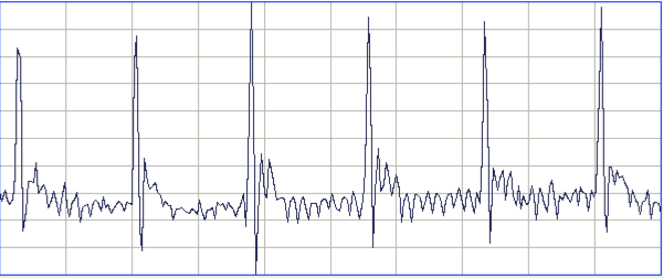
To obtain this recording, our collaborators at AMU cut the two ECG leads to the correct length, stretched the final 10 mm of the wire and insulation, then cut around the insulation 5 mm from the tip. The insulation pulls away from a 1-mm length of wire. They cover the tip with a silicone cap, which they hold in place with a 0/5 silk suture by squeezing the tip onto the lead.
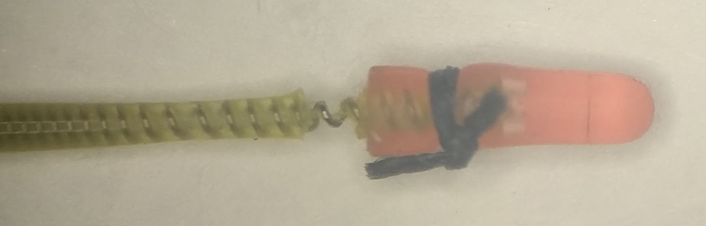
During surgery, they tie the exposed wire to the thoracic muscle with 0/5 sutures. One wire on one side of the heart, the other diagonally opposite.
[16-APR-18] We receive M1513090524.ndf from Edinburgh University, a recording made of intercostal muscles using an A3028B. We see heartbeat pulses, or electrocardiography, as well as respiration potential.

The figure below shows the spectrum of the combined respiration and heartbeat signal, in which the heartbeat and respiration can be distinguished. The heartbeat fundamental is at 6.3 Hz, with harmonics at 13 Hz and 19 Hz. Respiration fundamental is at 2.1 Hz with respiration second harmonic at 4.2 Hz.

Here is a four-second interval from a recording made by two electrodes running through an incision in the torso of an unconcious rat.

The heartbeat in the figure above, note the precise progression in the frequencies of the heartbeat harmonics, and the presence of the second harmonic of respireation. When we look at the spectrum from 0-10 Hz in more detail, we can see clearly the first, second, and third harmonics of respiration at 1, 2, and 3 Hz respectively. The fourth harmonic is too small to see, which is how we are able to detect both heartbeat and respiration in the same interval: the fundamental or heartbeat is much larger than the fourth harmonic of respiration.

We can measure heartbeat with the EKG1V2 interval processor using the Neuroplayer. This processor is a variation on our spike-finding algorithm. It counts the number of heartbeat spikes in the interval and fits a straight line to their positions so as to obtain an averager spike frequency, which we assume to be the heart rate. In addition, the processor high-pass filters the signal so as to remove the respiration potential, then calculates the average power of the signal between the EKG spikes.

For the above plot, we removed components below 10 Hz before using half the signal between each pair of EKG spikes to obtain our amplitude measurement. We have no reason to believe that the above inter-spike amplitude correlates well to EMG, but we provide the processor to calculate the inter-spike power in case anyone wants to try it.
[06-AUG-10] At CHB, we have transmitter No.6 implanted, with electrodes cemented to the skull by silver epoxy. We record 1000 seconds in archive M1281121460. At time 936 s, we observe seizure-like activity, even though the rat is not epileptic. We observe the rat chewing the sanitary sheets shortly before and after we notice the signal.

We put the rat in a cage within the enclosure. It roams around. We record 140 seconds in archive M1281122799. We again notice seizure-like activity at various times, including 104 s. We apply our seizure-finding algorithm. It does not identify any seizures. We apply the script to an older archive M1262395837 from ION and detect this seizure during the 4-s interval after time 1248 s. The amplitude of the ION signal is greater and the frequency of the oscillations is higher than in the CHB signal. Peak power is at around 10 Hz in this seizure, while we see no definite peak power in the seizure-like signal.
[08-AUG-10] Alex says the "recorded signal from our rat may be chewing artifact, but if I didn't have the history, I would say these are high voltage rhythmic spikes of Long Evans rats."
[12-AUG-10] In archive M1281455686 recorded by Sameer Dhamne (Children's Hospital Boston), we see EEG from implanted transmitters No8 and No10. At time 1140 s, Sameer's iPhone interferes with radio-frequency reception. Reception from No8 drops to 0%. Reception from No10 drops to 70%. In a 4-s interval we receive 25 bad messages on channel No5. There are a similar number of bad messages in channel No10. The bad messages produce a seizure-like spectrum, as shown below.
We modify our seizure-detection so that it looks for seizures only when reception is robust (more than 80% of messages received).
[20-AUG-10] The TPSPBP processor calculates reception, transient power, seizure power, and burst power simultaneously for all selected channels. We apply the script to six hours of data starting with archive M1281985381 and ending with archive M1282081048. The following graph shows transient and seizure power during the 21,000 second period.

We see transient and seizure power jumping up for periods of a few minutes, growing more intense as time goes by. According to our earlier work, a seizure is characterized by high seizure power and low transient power, so we doubt that these events are seizures. The peak of seizure power corresponds to the following plot of EEG.

The plot shows oscillations at around 3 Hz, but also a swinging baseline, which gives rise to the transient power. We are not sure if this is a seizure or not. Other examples of the signal with high seizure power show larger swings in the baseline, 0.5-Hz pulses, and rapid, but not instant, changes in baseline potential.
[25-AUG-10] Receive another six hours of data from Sameer Dhamne (Children's Hospital Boston), starting with archive M1282668620 and ending with M1282686620. The rat was less active and more asleep during these six hours. We plot signal power here. There are no seizure-like events.
[23-JAN-18] Suppose we have characteristics files that record the power in each of a set of frequency bands. Such characteristics are created by a processor like this:
append result "$info(channel_num) "
set f_lo 0.5
foreach f_hi {4.0 12.0 30.0 80.0 120.0 160.0} {
  set power [Neuroplayer_band_power [expr $f_lo + 0.01] $f_hi 0]
  append result "[format %.2f [expr 0.001 * $power]] "
  set f_lo $f_hi
}
You can download the above processor script as a text file by clicking here. The characteristics files contain lines like this:
M1435218371.ndf 28.0 14 1.44 1.65 1.47 3.10 0.58 0.37
M1435218371.ndf 29.0 14 6.40 1.95 1.33 2.52 0.74 0.29
M1435218371.ndf 30.0 14 0.62 2.81 1.52 3.34 0.48 0.58
M1435218371.ndf 31.0 14 3.50 1.29 1.15 2.64 0.92 0.48
M1435218371.ndf 32.0 14 1.82 1.05 1.55 3.73 0.47 0.32
The Power Band Average (PBAV4.tcl) interval analysis allows us to calculate the average or median power in each frequency band over a period greater than an interval, such as hourly or daily. We run the script in the Toolmaker and select our characteristics file. The analysis script produces another file containing the average powers in each averaging period.
[21-JAN-20] Here is a simple example of PBAV4.tcl in action. We have characteristics files with lines like this, where the single power band is the total power in 2-40 Hz recorded by an A3028P1-AA SCT implanted in a mouse.
M1576603629.ndf 136.0 53 8559.5
M1576603629.ndf 144.0 53 11230.9
M1576603629.ndf 152.0 53 12699.8
M1576603629.ndf 160.0 53 14412.7
M1576603629.ndf 168.0 53 13371.9
M1576603629.ndf 176.0 53 12112.7
We copy and paste the PBAV4 script into an empty Toolmaker window, and we set num_bands to 1, averaging_interval to 600, channel_select to 53, and calculation_type to 1 so that we obtain the median power in ten-minute intervals and write to disk with a timestamp. We select all 144 of our characteristics file and obtain a plot of median EEG power. We repeat with calculation_type set to 2 to obtain the maximum power. We plot the square root of the power multiplied by 0.41 μV to obtain the amplitude of the EEG versus time. The result is shown below.

The above experiment is a good check for electrode artifact: any ten minute interval with movement artifact in the EEG will show a maximum amplitude far greater than 100 μV.
[04-APR-11] Joost Heeroma (Institute of Neurology, UCL) asks us to provide a scripts that will calculate the average power in various frequency bands over a period of an hour. We start with a script that calculates the power in several bands of interest. The Power Band Average (PBA.tcl) script for use with the Toolmaker. The script opens a file browser window and we select the characteristics files from which we want to calculate power averages. With the parameters given at the top of the script, we instruct the analysis on how many power bands are in each channel entry, which channels we want to analyze, and the length of the averaging period. The averages appear in the Toolmaker execution window. We cut and paste them into a spreadsheet, where we obtain plots of average power in all available bands.

We used the power average script to obtain the above graph of mains hum amplitude versus time as recorded by Louise Upton (Oxford University) in her office window over ninety hours. We see the power averaged over one-minute periods. A twenty-four hour cycle is evident, and some dramatic event in which the transmitter was moved upon its window sill.
[07-FEB-20] The coastline of a signal is the sum of the distances from one sample to the next. If the signal is a voltage versus time, we tend to ignore the changes in time between the samples, and add only the absolute change in voltage between each sample. The normalized coastline is the coastline divided by the number of steps. The number of steps is the number of samples minus one. When the number of samples is large, we can ignore the minus one and just divide by the number of samples. The normalized coastline does not depend upon the size of our playback interval, so we can change the playback interval without having to re-interpret the normalized coastline. The figure below is a close-up of four EEG signals, showing the steps between samples.

The following processor calculates the normalized coastline, converts to μV with a scaling factor chosen to suit the transmitter, and adds the result to the processor's characteristics line.
set scale "0.41"
set coastline [format %.1f [expr \
	$scale*[lwdaq coastline_x $info(values)]/[llength $info(values)]]]
append result "$info(channel_num) [format %.1f [set coastline]] "
The figure below is an example of the coastline of EEG recorded from a mouse with a 40-Hz bandwidth subcutaneous transmitter.

When we change from eight-second intervals to half-second intervals, the value of normalized coastline does not change in proportion to the length of the interval, but instead we have the normalized coastline of an eight-second interval equal to the average of the normalized coastlines of all its sub-intervals.

The processor uses the lwdaq coastline_x library routine to calculate the coastline, then divides by the number of samples to get the normalized coastline. Other coastline routines available in LWDAQ are: lwdaq coastline_x_progress, lwdaq coastline_xy, lwdaq coastline_xy_progress.
[08-FEB-20] The correlation between two signals is a measure of how much they change together. For the purpose of comparing two EEG signals recorded from two different parts of the brain, we define correlation between X and Y across N samples to be the sum of products (Xn−Xn−1)*(Yn−Yn−1) for n = 2..N. If X changes by +6 from one sample to the next, while Y changes by −2 between the same two sample instants, the correlation between these two samples is −12. The normalized correlation is the correlation divided by the N−1. For large numbers of samples, we just divide by N.
Our dual-channel transmitters provide two signals, X is the odd channel number M, and Y is an even channel number M+1. The following processor detects whether it is acting upon X or Y. If X, it stores the signal values for later use. If Y, it assumes the existence of the stored X values and uses them to obtain the normalized correlation. It writes the X channel number and the normalized correlation to the result string.
set scale "0.41"
if {$info(channel_num) % 2 == 1} {
	set info(x_values) $info(values)
} {
	set correlation 0
	for {set i 1} {$i < [llength $info(x_values)]} {incr i} {
		set correlation [expr $correlation + \
			([lindex $info(x_values) $i]-[lindex $info(x_values) $i-1])\
			*([lindex $info(values) $i]-[lindex $info(values) $i-1])]
	}
	set correlation [expr $scale*$scale*$correlation/[llength $info(x_values)]]
	append result "[expr $info(channel_num) - 1] [format %.1f [expr $correlation]] "
}
The units of normalized correlation are square-cnt, or we can multiply twice by the transmitters scaling factor in μV/cnt to obtain correlation in μV2, which is what we do in the above processor.
[09-FEB-20] If we have a two-channel transmitter imlanted, we my want to look at the difference beteween the signal recorded by the two channels. The following processor obtains and plots the difference between X and Y recorded by a dual-channel transmitter, where X has an odd channel number M, and Y has an even channel number M+1. The processor uses the Neuroplayer_plot_values routine to display the difference signal in the value versus time plot. It also calculates the standard deviation of the difference signal and adds it to the characteristics line.
set scale "0.41"
if {$info(channel_num) % 2 == 1} {
	set info(x_values) $info(values)
} {
	set info(y_values) $info(values)
	set info(d_values) ""
	for {set i 0} {$i < [llength $info(values)]} {incr i} {
		append info(d_values) \
			"[expr [lindex $info(x_values) $i] - [lindex $info(y_values) $i]] "
	}
	Neuroplayer_plot_values [expr $info(channel_num) + 15] $info(d_values)
	scan [lwdaq ave_stdev $info(d_values)] %f%f%f%f%f ave stdev max min mad
	append result "[expr $info(channel_num) - 1] [format %.1f [expr $scale*$stdev]] "
}
The differences will be plotted in a color we calculate form the channel number by adding 15 to the channel number. This makes sure that the differences have a different color from the original X and Y.

If we want to obtain the coastline of the difference, we can take code from our coastline processor to obtain and print out the coastline of the differences.
[09-JUN-11] We have 67 hours of continuous recordings from two animals at CHB. Both animals have received an impact to their brains, and have developed epilepsy manifested in seizures of between one and four seconds duration. The transmitters are No4, and No5. The recordings cover 09-MAY-11 to 12-MAY-11 (archives M1304982132 to M1305220312). Our objective is to detect seizures with interval processing followed by interval analysis. The result will be a list of EEG events that we hope are seizures, giving the time of each seizure, its duration, some measure of its power, and an estimate of its spike frequency. The list should include at least 90% of the seizures that take place, and at the same time, 90% of the events in the list should be genuine seizures.
We sent a list of 105 candidate seizures on No4 to Sameer. He and Alex looked through the list declared 83 of them to be seizures, while the remaining 22 were not. On the basis of these examples, we devised our ESP1 epileptic seizure processor and our SD3 seizure detection.
 |
 |
 |
 |
 |
 |
The confirmed seizures all contain a series of spikes. The other seizure-like oscillations can be large, like confirmed seizures, but they do not contain spikes. In the Fourier transform of the signal, spikes manifest themselves as harmonics of the fundamental frequency, as we can see in the following plot of the signal and its transform.

The fundamental frequency of these short seizures varies from 5 Hz to 11 Hz. Because we want to measure the seizure duration to ±0.5 s, we must reduce our playback interval to 1 s. Thus our Fourier transform has components only every 1 Hz, and our frequency resolution will be ±0.5 Hz. Our first check for a seizure is to look at power in the range 20-40 Hz, which corresponds to the third and fourth harmonics of most seizures. Thus our seizure band is 20-40 Hz, not the 2-20 Hz we worked with initially. A 1-s interval is a candidate seizure if its seizure band amplitude exceeds 35 μV (which for the A3019D is 15 k-sq-counts in power).
We eliminate transient events by calculating the ratio of seizure power to transient power, with transient band 0.1-2.0 Hz. For the weakest seizures, we insist that the seizure power is four times the transient power. For stronger seizures, detection is less difficult, and we will accept transient power half the seizure power.
The final check for a seizure event is to confirm that it is indeed periodic with frequency between 5 Hz and 11 Hz. We find the peak of the spectrum in this range, and determine its amplitude. We require that the fundamental frequency amplitude be greater than 40 μV (which for the A3019D is 100 counts).
With these criteria applied to both the No4 and No5 recordings, we arrive at two lists of seizures, almost all of which contain spiky signals that we give every appearance of being seizures. There are 529 seizures in 67 hours on No4, and 637 seizures on No5. The CEL4V1 (Consolidate Event List Version 4.1) script reads an event list and consolidates consecutive events. The output is a list of consolidated events and their durations. See Event Consolidation for more details.
[17-JUN-14] Here is a history of our efforts to perform baseline calibration, which is to measure the power of normal, or baseline, activity in our recording so as to account for variations in the sensitivity of our recording device. The Neuroplayer provides support for baseline calibration. We have used with good effect on tens of thousands of hours of EEG recordings. Our first definition of baseline power in EEG was "minimum power", but this definition sometimes fails us. After epileptic seizures, EEG can be depressed to a power ten times lower the minimum we would observe in a healthy animal.
[09-JUN-11] The seizure-detector we presented in the section above used absolute power values as thresholds for the detection of seizure signals. The analysis will be effective with the recordings from multiple transmitters only if all transmitter electrodes are equally sensitive to the animal's EEG. In practice, we observe that the sensitivity of electrodes can vary by a factor of two from one animal to the next, as each animal grows, and in the final days of a transmitter's operating life.
Our study of baseline power above shows that during the course of sleeping and waking, a rat's EEG remains equal to or above a baseline power. The minimum power we observe is therefore a useful measure of baseline power. When we have a measure of baseline power, we can identify EEG events using the ratio of signal power to baseline power instead of the absolute signal power.
Our algorithm for baseline calibration is to as follows. First, we choose a frequency band that contains the power associated with the events we want to find. For seizures, we might choose 2-20 Hz as our event band. Looking at this graph we expect the minimum power in the event band to be around 4 k-square-counts for EEG recorded in a rat with an A3019D. When we start processing a recording, we set our baseline power to twice this expected value. As we process each playback interval, we compare the event power to our baseline power. If the event power is less, we set the baseline power to the new minimum. If the event power is greater, we increase the baseline power by a small fraction, say 0.01%. Increasing at 0.01%, the baseline power will double in two hours if it is not depressed again by a lower event power. The processor records the baseline power in the interval characteristics, so that subsequent analysis can have available to it the correct baseline power as obtained from the processing of hours of data.
By this algorithm, we hope to make our event detection independent of electrode and transmitter sensitivity. As a pair of electrodes becomes less sensitive with the thickening of a rat's skull, we reduce our baseline power through the observation of lower and lower event power. As a transmitter becomes more sensitive with the exhaustion of its battery, the fractional growth of our baseline power allows us to find the new minimum event power.
[26-NOV-12] The Neuroplayer provides baseline power variables for processor scripts to use. The baseline power for channel n should be stored in info(bp_n). We can edit and view the baseline powers using the Neuroplayer's Baselines button. We implement our baseline calibration algorithm in the BPC1 processor, where we use the baseline power variables in the processor script.
[15-APR-14] We have recordings of visual cortex seizures from ION, both single and dual channel. The following plot shows the minimum and average hourly power measured in eight-second intervals during 450 hours of recording from transmitter No8, M1361557835.ndf through M1367821007.ndf recorded in the ION bench rig.

At time 191 hr, the minimum power drops to 1.3 k-sq-counts while the average power remains around 30 k-sq-counts. During this hour, the reception is excellent, and the animal is having seizures. At 410 hours, the average power has risen to 200 k-sq-counts while minimum power drops to 1.13 k-sq-counts. But in this period, there are two No8 transmitters operating, and one of them is showing large transient pulses. The distribution of eight-second playback interval power during the entire 450-hour recording is shown here.
[02-JUN-14] In the figure above, there are several hours in which the minimum EEG power drops far below what is usual. At time 191 hr the minimum power is 1.3 k-sq-counts. There is one interval in which EEG appears to be depressed after an extended seizure.

A depressed interval drops our baseline power to the point where almost all subsequent intervals exceed our threshold for event detection. We found several such intervals in the same hour. The majority of the hour was occupied by vigorous epileptic activity like this.
Meanwhile, the power of the electrical noise on the transmitter input increases with the impedance of the electrodes. In the extreme case, when the electrode leads break near the electrode, the noise looks like this. The figure below shows an eight seconds of normal mouse EEG recorded with M0.5 screws.

The spectrum of this interval is 1/f (pink) from 1-20 Hz and constant (white) from 20-160 Hz. The pink part reaches an amplitude four times higher than the white part. In the depressed rat EEG interval, the pink region is also 1-20 Hz, but the pink part reaches an amplitude twenty times higher than the white part. The spectrum of the baseline signal affects our choice of event power threshold, because white noise power varies far less than pink noise power over a finite interval of time. In mice we use a threshold of three times the baseline power, while in rats we use five times.
The existence of depressed intervals upsets our use of minimum power for our baseline calibration. The fact that the lowest-power intervals can be interesting upsets our use of high power as our trigger for event classification. The fact that the spectrum of noise varies with animal species and electrode size makes our power threshold dependent upon these factors also. The baseline calibration we have attempted to implement may be impractical. We are not even sure we can agree upon the definition of baseline power. We are considering abandoning baseline power calibration and replacing it with a straightforward, absolute, logarithmic power metric.
[09-JUN-14] Here is an absolute power metric that covers the full dynamic range of our subcutaneous transmitters.

The metric, power_m, is a sigmoidal function of signal power, P, where P is in units of k-sq-counts. We have P_m = 1 / (1 + (P/100.0)−0.5). Its slope is greatest at 100 k-sq counts, or 90 μV rms in the A3028A transmitter, which is the root mean square amplitude of typical seizures.
[22-DEC-14] With the metrics of the ECP11V3 event classification processor, we can distinguish between healthy, baseline EEG and post-seizure depression EEG, without using a power metric. We see superb separation of depression and baseline events with coastline and intermittency metric here (Depression is light blue, Baseline is gray). Both metrics are normalized with respect to signal power. Our plan now is to identify baseline intervals and measure their minimum power so as to obtain our baseline calibration. Our calibration will affect the constant in the above sigmoidal function, so as to bring baseline intervals into the metric range 0.2-0.4, allowing us to use a power metric threshold of 0.4 to eliminate almost all baseline intervals and so make correct identification of seizure and other artifacts more likely. We present this scheme below in Event Classification with ECP11.
[23-FEB-12] Readers may dispute the classification of EEG events as "eating" or "hiss" or "seizure" in the following passage. We do not stand by the veracity of these classification. Our objective is to demonstrate our ability to distinguish between classes of events. We could equally well use the names "A", "B", and "C".
[08-AUG-08] The following figure presents three examples each of hiss and eating events in the EEG signal recorded with an A3019D implanted in a rat. We are working with the signal from channel No4 in archive M1300924251, which we received from Rob Wykes (Institute of Neurology, UCL). This animal has been injected with tetanus toxin, and we assume it to be epileptic.
 |
 |
 |
 |
 |
 |
Hiss events are periods of between half a second and ten seconds during which the power of the signal in the high-frequency band (60-160 Hz) jumps up by a factor of ten. We observe these events to be far more frequent in epileptic animals, and we would like to identify, count, and quantify them. The eating events occur when the animal is chewing. Eating events also exhibit increased power in the high-frequency band, but they are dominated by a fundamental harmonic between 4 and 12 Hz.
Our job is to identify and distinguish between hiss and eating events automatically with processing and analysis. We find our task is complicated by the presence of three other events in the recording: transients, rhythms, and spikes.
 |
 |
A transient event is a large swing in the signal. A spike event is a periodic sequence of spikes, which we suspect are noise, but might be some form of seizure. A rhythm is a low-frequency rumble with no high-frequency content. For most of the time, the EEG signal exhibits a rhythm that is obvious as a peak in the frequency spectrum between 4 and 12 Hz, but sometimes this rhythm increases in amplitude so that its power is sufficient to trigger our event detection.
The Event Detector and Identifier Version 2, EDIP2, processor detects and attempts to distinguish between these five events. Read the comments in the code for a detailed description of its operation. The processor implements the baseline calibration algorithm we describe above. It is designed to work with 1-s playback intervals. In addition to calculating characteristics, the processor performs event detection and identification analysis immediately, so that you can see the result of analysis as you peruse an archive with the processor enabled.
The processor defines four frequency bands: transient (1-3 Hz), event (4-160 Hz), low-frequency (4-16 Hz), and high-frequency (60-160 Hz). When the event power is five times the baseline power, the processor detects an event. The processor records to the characteristics line the power in each of these bands. These proved insufficient, however, to distinguish eating from hiss events, so we added the power of the fundamental frequency, just as we did for our detection of Short Seizures.
These characteristics were still insufficient to distinguish between spike and eating events, so we added a new characteristics called spikiness. Spikiness is the ratio of the amplitude of the signal in the event band before and after we have removed all samples more than two standard deviations from the mean. Thus a signal with spikes will have a high spikiness because the extremes of the spikes, which contribute disproportionately to the amplitude, are more than two standard deviations from the mean. We find that baseline EEG has spikiness 1.1 to 1.2. White noise would have spikiness 1.07. Eating events have spikiness 1.2 to 1.5. Spike events are between 1.5 and 2.0. Hiss events are between 1.1 and 1.3. Thus spikiness gives us a reliable way to identify spike events.
The processor uses the ratio of powers in the various bands, and ranges of spikiness, to identify events. After analyzing the hour-long recording and examining the detected events, we believe it to be over 95% accurate in identifying and distinguishing hiss and eating events. Nevertheless, the processor remains confused in some intervals, such as those we show below.
 |
 |
 |
The processor does a good job of counting hiss and eating events in an animal treated with tetanus toxin. We are confident it will perform well enough in control animals and in other animals treated with tetanus toxin.
[10-AUG-11] Despite the success of the Epileptic Seizure Processor Version 1, ESP1, and the Event Detector and Identifier processor Version 2, EDIP2, we are dissatisfied with the principles of event identification we applied in both processors. It took many hours to adjust the identification criteria to the point where their performance was adequate. Furthermore, we find that we are unable to add the detection of short seizures to the processor, nor the detection of transient-like seizures we observe in recent recordings from epileptic mice.
[03-JUN-19] The Event Classifier provides us with a way to identify events automatically by comparing them to events we have classified with our own eyes. Our Event Classification Processor Version 1 (ECP1) produces eight characteristics for each channel. The first is a letter code that we can use to mark likely intervals at the time of processing. The second is the baseline power, which we obtain from the processor's built-in baseline calibration. The remaining six are values between zero and one that we call metrics. The metrics are characteristics of the interval. Our newer event classification processors are similar, but their metrics are superior, see ECP20V2 and Event Classification with ECP20. In the paragraphs below, we present the principles of classification by similarty using the ECP1 processor.
Of the six metrics, the first is the power metric. If the events we are looking for are more powerful than baseline events, as is the case with many forms of epileptic seizure in EEG, we have the option of using the power metric to make a first selection of intervals for classification. When the power metric is higher than a threshold we decide upon, we will attempt to classify the event as, for example, ictal, spike, grooming, or artifact. In recent years, however, we have tried wherever possible to avoid using the power metric for classification. To calculate the power metric, we must divide the amplitude of the signal by some our best estimate of the amplitude of the baseline signal. This estimate can be hard to obtain. The amplitude of baseline EEG recorded from skull screws varies from one pair of skull screws to another. The amplitude can vary with time as scar tissue grows over the ends of the screws. Our efforts to determine the baseline amplitude automatically have been defeated by recordings in which an animal has seizures for most of an hour, and then has periods of depression where the amplitude is much lower than that of normal EEG.
The metrics produced by ECP1 are event power, transient power, high-frequency power, spikiness, asymmetry, and intermittency. Event power is a sigmoidal function of the ratio of the power in the 4.0-160.0 Hz band to the baseline power, with a ratio of 5.0 giving us a metric of 0.5. Transient power is a sigmoidal function of the ratio of power in the 1-3 Hz band to the baseline power, with a ratio of 5.0 giving us a metric of 0.5. High-frequency power is a sigmoidal function of the ratio of power in the 60-160 Hz band to power in the 4.0-160 Hz band, with a ratio of 0.1 giving us a metric of 0.5. Spikiness is a sigmoidal function of the ratio of the range of the 4.0-160.0 Hz signal to its standard deviation, with a ratio of 8.0 giving us a metric of 0.5. Asymmetry is a sigmoidal function of the number of points more than two standard deviations above and below the mean in the 4.0-160 Hz signal. When these numbers are equal, the asymmetry is 0.5. When the number above is greater, the asymmetry is greater than 0.5. Thus downward spikes give us asymmetry of less than 0.5. The intermittency metric is a measure of how much the high-frequency content of the signal is appearing and disappearing during the course of the interval. We rectify the 60-160 Hz signal, so that negative values become positive, then take the Fourier transform of this rectified signal. The power in the 4.0-16.0 Hz band of this new transform is our measure of intermittency power. Our intermittency metric is a sigmoidal function of the ratio of intermittency power to high frequency power. The metric has value 0.5 when the intermittency power is one tenth the power in the original 60-160 Hz signal.
All six of these metrics are invertible, in that we can recover the original event, transient, high-frequency, and intermittency powers, as well as the spikiness and asymmetry by inverting the sigmoidal functions with the help of the baseline power. An example of a Toolmaker script that performs such an inversion is CMT1.
The Event Classifier allows us to build up a library of events that we have classified visually. Once we have a large enough library, we use the metrics to compare test events with the reference events. The reference event that is most simliar to the test event gives us the classification of the test event. If the nearest event is a hiss event, we assume the test event is a hiss event also. Our measure of the difference between two events is the square root of the sum of the squares of the differences between their metrics.
With six metrics, such as produced by the ECP1 classification processor, we can imagine each event as a point in a six-dimensional space. The difference between two events is the length of the six-dimensional vector between them. Because metrics are bounded between zero and one, the Classifier works entirely within the unit cube of our six-dimensional space. We call this unit cube the classification space. A test event appears in the classification space space along with the reference events from our library. We assume the test event is of the same type as its nearest neighbor.
The map provided by the Event Classifier shows us a projection of the classification space into a two-dimensional unit square defined by the x and y metrics selected by the user for the map map. We see the reference events as points, and the test event also. By selecting different projections, we can get some idea of how well the metrics are able to separate events of different types. But the picture we obtain from a two-dimensional projection of a higher-dimensional classification space will never be complete. Even with three metrics, we could have events of type A forming a spherical shell, with events of type B clustered near the center of the shell. In this case, our projections would always show us the B events right in the middle and among the A events, but the Classifier would have no trouble distinguishing the two by means of its distance comparison.
We apply ECP1 and the Event Classifier to archives M1300920651 and M1300924251, which we analyzed previously in Eating and Hiss. You will find the ECP1 characteristics files here and here. These archives contain signals from implanted transmitters 3, 4, 5, 8, and 11. We build up a library of a hundred reference events using No4 only. The library contains hiss, eating, spike, transient, and rhythm events as we showed above. Also in the library are rumble events, which are like rhythms but less periodic. Some events are a mixture of two overlapping types, and when neither is dominant we resort to calling them other. We find the same dramatic combination of downward transient, hiss, and upward spikes a dozen times in the No4 recording, and we label these seizure.
 |
 |
 |
We apply Batch Classification to the entire two hours of recording from no4, classifying each of two thousand one-second events using our library of one hundred reference events. We go through several hundred of the classified events and find that the classification is correct 95% of the time. The remaining 5% of the time are events whose appearance is ambiguous, so that we find ourselves going back and forth in our visual classification. The Classification never fails on events that are obviously of one type or another.
We apply our reference library to the recording of No3. We add a few new reference events to describe transients suffered by No3 but not by No4. After this, we obtain over 95% accuracy on No3, as with No4. For No5 we add some surge events not seen on No4, and for No11 we add more eating events because this transmitter sees eating artifact upside down compared to the other channels, suggesting its electrodes were reversed. We also observe some seizure-like rhythm events, and we add a couple of examples of these to the library. We do not need to add new events to classify No8. You will find our final library here.
 |
 |
Transmitter No11's baseline power is only 0.5 k-sq-c compared to No3's 3.4 k-sq-c, meaning the baseline EEG amplitude is less than half that of No3. But the baseline calibration provided by ECP1 overcomes this dramatic difference, and we find our reference library is effective at classification in No11.
We repeat our classification procedure on our short seizure recording, which contains data from two transmitters, No4 and No5. Both animals show frequency powerful rhythm events, but No4 contains far more seizures than no5. These rhythms and seizures have a low proportion of high-frequency power. But the rhythm events tend to be symmetric, while the seizure events are downward-pointing. It is the asymmetry metric that allows us to distinguish between the two. With a library of only thirty-five events, we obtain over 95% accuracy at distinguishing between seizures and rhythms. Indeed, out of hundreds of rhythm events, only one or two are mistaken for seizures, and event then, we're not certain ourselves that these unusual events are not seizures.
Upon two entirely independent data sets, our method of similar events proves itself to by over 95% accurate. In once case it succeeded in classifying thousands of events from five transmitters into nine different types. In another case it distinguished between rhythms and short seizures with no difficulty.
[04-JAN-12] When we look at the Fourier transform of a signal, we are almost always looking at the amplitude of the components plotted against frequency. We call this the spectrum of the signal. It is almost impossible for the human eye to make sense of the graph of phase plotted against frequency. Nevertheless, this second graph is essential to the transform. When we ignore it, we are throwing away precisely half of the information contained in the transform. When we look at pendulum waves, for example, we see how the same frequency oscillations combine to give a wide variety of patterns depending upon their relative phases.
Thus the spectrum of a signal is not unique to the signal. There will be many signals with almost exactly the same spectrum, even though the original signals are dramatically different in their appearance. When we use the spectrum alone to detect events, we may find that we cannot distinguish between the events we are looking for and a far larger number of irrelevant events that have the same spectrum. In this section we present examples of how the Fourier transform can be misused when applied to EEG.
In the introduction to Unsupervised Classification of High-Frequency Oscillations in Human Neocortical Epilepsy and Control Patients (Blanco et al., Journal of Neurophysiology 104: 2900Ð2912, 2010), the authors write, "In the epilepsy research community, there is mounting interest in the idea that high-frequency oscillations (HFOs) − narrowband transients recorded on the intracranial electro-encephalogram (iEEG), having predominant frequency between roughly 100 and 500 Hz and lasting on the order of tens of milliseconds − can be used to identify epileptogenic brain tissue." To find these HFOs in their own recordings, they use a procedure similar to our Event Classifier, with metrics that rely partly upon the Fourier transform of the signal and partly upon non-linear features of the signal. At ION, our collaborators are working on detecting HFOs in human EEG, and they are wondering if looking at the power in various narrow bands between 100 Hz and 500 Hz will suffice as a detection mechanism. The following plot is a 2-s segment of four channels of a human EEG recording we received from ION (Institute of Neurology, UCL, Dr. Walker and Ms. Lemesiou).

We now take the central 1 s of the above recording, which contains some rapid fluctuations. We have 512 samples from each of the four channels. We take the discrete Fourier transform of the signal for each channel, remove all components below 80 Hz and above 200 Hz, then take the inverse transform.

The impression one might get from the above plot is that there are 100 Hz oscillations in the signal. But here is the same signal band-pass filtered to 40-200 Hz.

There are no 100 Hz oscillations. The signal contains oscillations of roughly 50 Hz. These vary in frequency during the one-second interval. These oscillations are asymmetric. In the Fourier transform, frequency variation and waveform asymmetry manifest themselves as frequency components at double the oscillation frequency. We call these double-frequency components the "second harmonics". The main, 50 Hz, components are the "fundamental frequencies" or "first harmonics". If you remove the first harmonics you are, of course, left with the second and higher harmonics. Here is the same EEG interval filtered to 120-200 Hz.

Here is a 64-Hz square wave we imported into the Neuroplayer. You can see the spectrum of the oscillation on the right, and on the left the oscillation itself in green. We plot the third harmonics on its own in purple. We extracted them with a 160-180 Hz band-pass filter.There is no second harmonic because the waveform is symmetric. But there is a third harmonic because the edges of the oscillation are sharp.

We cannot use bandpass filters to deduce the presence of oscillations at a particular frequency. By definition, a harmonic is not an oscillation. The oscillation is the sum of all the harmonics. These harmonics emerge when we transform the original signal into an abstract place called the "frequency domain". We are permitted to say that there are "oscillations at 100 Hz" only if there is no fundamental harmonic at 50 Hz.
[22-MAR-12] In Pitfalls of high-pass filtering for detection of epileptic oscillations, Clinical Neurophysiology, 2010, Benar et al. make the same argument we present above. In Continuous high-frequency activity in mesial temporal lobe structures, Epilepsia, 2012, Mari et al. apply an 80-Hz high-pass filter to epileptic human EEG and observe continuous high-frequency oscillations in the output of the filter. The examples below show how this will always be the case. We take one second of EEG from a non-epileptic, active mouse (recorded at Oxford University, 25-JUL-11, archive M1311606907, we picked 40-41 s at random) and apply three sharp high-pass filters: 40 Hz, 60 Hz, and 80 Hz. In each case, we see the apparent frequency of oscillation is about 20 Hz above the filter cut-off frequency.


When we apply a step function to a filter, its output will ring afterwards, at a frequency close to the cut-off frequency. The ringing continues for longer as the filter gets sharper.


Filters with a more gentle cut-off produce ringing of smaller amplitude that decays more quickly. The images above show the same data we presented above, with the same cut-off frequencies, except that the high-pass filter allows a fraction of components less than 20 Hz below the cut-off frequency to remain in the filtered signal. The frequency response of the filter, in terms of amplitude, looks like a straight line from zero at 20 Hz below the cut-off, to one at the cut-off. Despite the gentle nature of this filter, we see that the same filter-generated oscillations remain in the signal.
[15-JAN-12] In the previous section we showed that the Fourier transform's amplitude spectrum alone was insufficient to identify high-frequency oscillations (HFOs) in EEG. In general, no matter what the appearance of the original signal, there will be other signals of dramatically different appearance with exactly the same amplitude spectrum. Their Fourier transforms are distinguished by the phases of their frequency components, not by the amplitudes. Thus the amplitude spectrum is not an adequate representation of the EEG signal for the identification of HFOs. In this section we present general-purpose definition of adequate representation that applies equally well to our Event Classifier and the Fourier spectrum.
Suppose we have an interval of EEG or some other signal, made up of M samples. Each sample xi has a one-dimensional value. In the case of the SCT system, the samples have integer values between 0 and 65535 as produced by the sixteen-bit analog to digital converters on the transmitters. We can think of each interval as being a point, x, in an M-dimensional space. Let S be the set of all possible intervals. In the case of the SCT system, S is an M-dimensional cube of side 65535 with one corner at the origin.
Let A ⊂ S represent the set of all intervals of a particular type. Thus A might represent the set of all intervals that contain one or more HFOs, or it might represent the set of all intervals that contain seizure spikes. For any interval x ∈ S, we can examine the interval ourselves and determine whether x is in A or not. In the SCT system, we would look at x as it appears in the voltage versus time plot of the Neuroplayer. Complimentary to A, we have a set S−A which contains all intervals that are not members of A. Obviously, A ∪ S−A = S and A ∪ S−A = ∅.
Our objective is to pick out from a large number of intervals those that are members of A. We can do this by eye, but it takes several seconds per interval, and if we have a million intervals, the task becomes impractical. Thus we set out to perform the classification with a computer. This we do by transforming each interval into another form, and classifying the interval based upon some simple proximity or threshold rules we apply to this other form. In general, we transform points in S into points in another space T. In Similarity of Events we transform 512 consecutive sixteen-bit samples into six real-valued metrics, each of which is a number between zero and one. Thus T is a six-dimensional unit cube with one corner at the origin. In Harmonics and Fundamentals we transform 512 consecutive sixteen-bit samples into 256 components of an amplitude spectrum. Thus T is a 256-dimensional cube with one corner at the origin. (The sides of this cube have length 65535 × √2, but that's not so obvious.)
Let F be a function such that for any x ∈ S we have y = F(x) is the transform of x, with y ∈ T. We call F our transform function. Furthermore, we write F(A) to represent the set of all points y ∈ T such that there exists x ∈ A for which y = F(x). Thus F(A) is the transformed version of A. In the same way, F(S−A) is the transformed version of S−A.
The discrete Fourier transform of an interval, including both amplitude and phase information, is a one-to-one transformation of points in the time domain, S, into points in the frequency domain, T. Given any point in T we can deduce the one and only point in S from which that point could arise. The function F is invertible, which is to say that F−1(y) exists, where F−1(F(x)) = x. If we use only the amplitude spectrum of the Fourier transform, however, the transformation is no longer one-to-one. The function F−1(y) does not exist, and for any y ∈ T there are many x ∈ S such that F(x) = y. When we transform intervals into six metrics, it is clear that we cannot deduce the original signal from the transformed point. What we can hope for, however, is that y = F(x) contains enough information for us to deduce whether or not x ∈ A.
By construction, we have A ∩ S−A = ∅ and A ∪ S−A = S. We don't care if F(A) ∪ F(S−A) = F(S) = T. Indeed, when we restrict S to a finite number of recorded intervals, we will find that F(S) is a proper subset of T. But we certainly prefer to have F(A) ∩ F(S−A) = ∅. If not, there exist points y ∈ F(A) ∩ F(S−A) such that y is the transform of at least one point in A and one point in S−A. In other words, we cannot use y to determine if x ∈ A. We say F is ambiguous with respect to A. The set of points x ∈ S such that F(x) ∈ F(A) ∩ F(S−A) is the ambiguous region of S with respect to A. The set F(A) ∩ F(S−A) is the ambiguous region of T with respect to A.
If we are to use F to determine if x ∈ A, the function must be unambiguous with respect to A. If F is invertible, then it will certainly be unambiguous with respect to A. But we want to work with functions that greatly reduce the amount of information our computer must deal with when applying our classification rules. In that case, F will not be invertible. We can, however, prove that F is unambiguous with respect to A by going through all members of S, inspecting each by eye, transforming them, and constructing the ambiguous region of S with respect to A. If this region is empty, then F is unambiguous with respect to A.
But in practice, S will contain too many members for us to inspect all of them. If S is the set of all possible combinations of 512 sixteen-bit samples, for example, it will contain 65536512 points. Even if we restrict S to the set of all such combinations that we have actually recorded from a laboratory animal, the number of points in S will still be too large, because our original motivation for applying F to S was that it would take too much effort to inspect each and every point in S. In practice, therefore, F will not be invertible and it will be impractical to classify all members of S by visual inspection. But the requirement that F be unambiguous with respect to A remains.
Thus we need a practical procedure to show that F is unambiguous with respect to A. To do this, we will assume that S contains a finite number of points. This will indeed be the case in practice, even if that finite number is tens of millions of seconds of recorded signal. We now place further conditions upon F. Loosely speaking, we require that F be such that we can define F(A) with a finite set of spheres. In more precise language, F must be such that there exists a finite set of points L ⊂ T and a radius r > 0 such that the union of all spheres of radius r centered on the members of L, which we will call U, is such that F(A) ⊂ U and F(S−A) ∩ U = ∅. When such an L and r exist, we say that F separates A, and that U provides an adequate representation of A in F. We see that F separates A implies that F is unambiguous with respect to A.
Our task, therefore, is to find an adequate representation of A in F, because if we can do that we show at once that F is unambiguous with respect to A and we know F can separate A from S−A. Given any x ∈ S, we check to see if F(x) ∈ U, where U is our adequate representation of A in F, and if so, we know x ∈ A, but if not, we know x ∈ S−A.
In certain cases, we may find that there are other ways to determine if F(x) ∈ U besides going through all the spheres of U and checking to see if it contains F(x). For example, if one of our metrics is high-frequency power and another is intermittency, we might say that x is an HFO if the high-frequency power, intermittency, and purity of the signal all exceed certain thresholds, or lie within certain bounds. But it could be that the threshold for high-frequency power should be a function of the intermittency, in which case our fixed-threshold classification would perform poorly. Even if constant thresholds could give us effective classification, we would still be left with the task of determining the values of the thresholds. Indeed, after many hours spend adjusting such thresholds, we concluded that classification with constant thresholds is impractical.
We are left with the task of composing a list of points, L ⊂ T, and choosing a radius, r, that together will provide us with an adequate representation of A in F. Consider the following separation algorithm.
If it is true that F separates A, this algorithm will eventually provide us with an adequate representation of A in F. If we find, after inspecting a sufficiently large number of points in S, that r has converged to some final value, and we are no longer adding points to L, we can be confident that we have an adequate representation. We will not be certain, but we can at least be confident.
In the case where A is a very small subset of S, such as when we are looking for rare features in a recorded signal, our algorithm is not efficient in its use of inspector time. It requires the inspector to examine a large number of uninteresting events. If possible, we should devise some simple criterion for initial rejection before inspection. The Event Classifier, for example, uses its first metric for initial rejection. If this metric is less than one half, the Event Classifier assumes that the interval is not an event (it assumes x ∉ A). Furthermore, the algorithm is inefficient in its use of the points in L because it allows them to extend influence only over a distance r. The Event Classifier overcomes this inefficiency by using a nearest-neighbor search through L to determine if F(x) ∈ F(A) or F(x) ∈ F(S−A). Thus the points in L have influence over all points in S to which they are nearest, and therefore all points in S are included in the sphere of influence of at least one member of L.
[20-JAN-12] We would like to detect wave packets of center-frequency 100-200 Hz in human EEG recordings. In the epilepsy community, these wave packets are called HFOs (high-frequency oscillations). Our sample EEG recordings are provided by Athena Lemesiou (Institute of Neurology, UCL). They come from intracranial electrodes implanted in the brains of adult patients with epilepsy. The recordings contain seizures, rumble, and mains hum. On some channels we see one or two HFOs per minute, but on others we see none. We would like to ignore the non-HFO features and extract from the signal the wave packets. At the same time, we are aware of how easily we can create wave packets by the action of high-pass filtering, as we discuss above. We resolve not to classify the EEG intervals by looking at a filtered version of the signal. We will look at the original signal.

Although we will not use filtering in our visual identification of HFOs, we will use the power in the 80-260 Hz band to pick out intervals that might be HFOs. These intervals will be our events and the 80-260 Hz band will be our event band. Our hope is that we can train a computer to classify events as HFO or non-HFO. The upper limit of 260 Hz makes no sense for signals recorded at 512 SPS, but in this case our EEG data was recorded at 1024 SPS and filtered to 268 Hz. The power of our HFOs should lie entirely within the event band. We will use event-band power for baseline calibration. Our event-power metric is a measure of the ratio of the event power to the baseline power. After some examination of the data, we set our event trigger at ten times the baseline power.
We found that symmetry and spikiness were not useful in detecting HFOs, neither when applied to the 80-260 Hz signal nor to the 10-40 Hz signal. But intermittency remains useful, this being the power of fluctuations in the de-modulated event-band signal. We devised a new metric to measure the purity of a wave packet. A wave packet has a gaussian-shaped frequency spectrum. Our purity metric is a measure of how narrow this peak is compared to its center frequency. A sustained sinusoid will have maximum purity and a spike will have minimum purity. A wave packet is somewhere in-between.
Our ECP2 classification processor implements these three metrics. In the figure below we see a classification library arranged by purity and intermittency. The other two combinations of metrics give similar separation of HFO and Other events. All three metrics are necessary for adequate separation of the two classes.

We built up our classification library by starting with channel No1 in an archive P9_HG_N4_REF_1.ndf for which ION had confirmed twelve HFOs. We used six of these in our library three others we found ourselves. We included twenty Other events from channel No1. We applied the library to all fourteen channels in the same archive. We found 5 New events and classified these. We applied the library again. We found 0 New events, 24 HFO, and 175 Other. Going through the 24 HFO events we find they all match our visual criteria. Our false positive rate among detected HFO events is less than 1/24 = 4%. Our false positive rate among randomly-selected 0.5-s intervals is less than 1/16800 = 0.006%. Going through the 175 Other events, we find seven or eight that we think should have been classified as HFO. These are either too close to the edge of the interval or accompanied by large artifacts that make detection difficult. Because we have roughly 32 HFO events and we miss 8 of them our false negative rate is 25%.
[23-NOV-18] The Batch Classifier generates lists of events, each of which is one playback interval long. With a one-second interval, a one-minute seizure may appear as sixty consecutive ictal events in an event list. Or the seizure might begin with four ictal events, and end with the first stretch of four non-ictal events. A feeding session could consist of five consecutive chewing events and end when we have ten consecutive non-chewing intervals. Making a list of such longer-term events, each of which consists of many interval-length events, is what we call event consolidation.
Our CEL4V1 program (Consolidate Event List V4.1) is a LWDAQ Toolmaker script. Open the Toolmaker in the Tool Menu, press Load, and select the script file. Press Execute. The following window opens.

We read an event list with the read_events button. A file browser window opens up. The event list should be one produced by the Batch Classifier. We let the program know the interval length used for event classification with the interval_length parameter, which has units seconds.
Our event list can contain events from any number of channels. The CEL4 selects events arising on one particular channel number we specify in channel_id. If we want to include events from two different channels in our consolidation, perhaps because we are using a dual-channel transmitter and an ictal event on either should count towards a seizure, we use an earlier version of the consolidator, CEL3V2, which uses all events in a list regardless of channel number. We have the Batch Classifier write a list of all events from the channels that we want to include, and apply CEL3V2 to this list.
The CEL4V1 and CEL3V2 consolidation algorithms begin by looking for a minimum number of consecutive events in the list. If we set min_start_intervals to 5, any sequence of five events in consecutive playback intervals marks the start of a consolidated event, and the start time will be the time of the first interval.
The consolidator's criterion for the termination of a consolidated event is the occurrence of more than a maximum number of break intervals during the consolidated event. If we set max_break_intervals to 4, then 5 consecutive playback intervals that do not contain an event will cause CEL2 to complete the current event, with the end of the consolidated event being the end of the final event it contains.
The event list written by the consolidator uses a ten-digit UNIX timestamp to mark the start time of the event, plus a fractional offset if such is necessary to get to the exact start time. Following the offset is the channel number of the first event in the consolidated event, its type, and the event duration. The name of the consolidated list we compose from the original event list, by adding a suffix, which you can specify with the consolidated_suffix parameter.
Example: We use Library_03FEB15 and ECP15V3 to produce a list of one-second ictal events in six separate hours of dentate gyrus field potential in a rat. We two hours before perforant pathway stimulation and several hours afterwards, not contiguous. We apply the consolidator, asking for five consecutive interval events to start a seizure and allowing no more than four break intervals. We obtain seven events in the recordings after stimulation and none in the recordings before. If we increase the minimum start events to ten, we get only one seizure, which is the one identified as the first seizure after stimulation by the group making the recordings (Philipps University, Marbug).
In the Neuroplayer, select the consolidated list in the Event Navigator. Step through the consolidated events to view them. Note that you can view the events with a longer playback interval than was used to obtain the original list of short events. If we use one-second intervals to make a list of ictal events, for example, we can view the consolidated events with 16-s intervals to see the evolution of a seizure on a longer timescale.
[19-MAY-17] Our new spike-finding algorithm SCPP4V1 is not fooled by the kind of step-changes in EEG that are generated by the movement of imperfectly-secured electrodes.x We plot our EEG signal as a sequence of points on a two-dimensional map. The grid squares of the map are one sample period wide. For a 512 SPS signal, the map squares are 1/512 s wide. The squares are one mean absolute step size high, where the mean absolute step size is the one-dimensional coastline of the signal divided by the number of samples. For baseline mouse EEG recorded with a skull screw, the map squares will be roughly 15 μV high.
We move along the EEG path in discrete steps. Each step moves us to a later point in the EEG signal. We try to make the step as small as possible. If we can take a smaller step by skipping one or more points, we do so. Points that we skip represent abberations from the path traced by the EEG signal. Our measure of the size of an aberration is the greatest distance from the aberration to the point we step to. We see the path-tracing in action below.

When the size of the aberration is greater than our spike_threshold, we classify the aberration as a spike. The threshold has units of mean absolute step size. A threshold of 20 works well to find spikes in transgenic mouse EEG. In the figure below we see how a step-artifact does not generate a spike detection with the path-finding algorithm.

We enhance the spike-finding by limiting the number of points we are permitted to skip when taking a step along the path. This number is the spike_extent. An extent of ten forces the path-tracer to follow any aberration that is more than ten samples long. Inter-ictal spikes recorded in mice at 512 SPS are less than ten samples long, but electrode artifact spikes are more than ten samples long. The M1445359478 archive, from University of Edinburgh, is notable for its 30-mV movement artifacts in channel No5 as well as a variety of smaller movement artifacts. To test how well we can find spikes in all manner of intervals, we inserted an artificial 700-μV spike in our data as we went through archive M1445359478 in 8-s intervals.


Out of 450 intervals in the M1445359478 archive, there are only one interval in which we do not find the artificial spike. In this interval, which we show in the figure above, huge artifacts have so greatly increased the mean absolute step size that the spike does not exceed our threshold. Our false negative rate on this archive is 1/450.
We use the SCPP4V1 processor to measure delta power (0.1-3.9 Hz) and count spikes in each 8-s interval of M1445359478. We sort the intervals in order of decreasing delta power. All intervals with delta power >100 ksq-counts (90 μV rms) contain some kind of movement artifact. We look at all these intervals and count false spikes, which are all caused by edges and features on artifacts, and actual spikes among the artifacts. We do this same experiment for spike thresholds 10 and 20. Considering the 27 intervals with delta power >100 ksq-counts, there are no obvious inter-ictal spikes we miss with either threshold 10 or 20.

We repeat this experiment with M1436545502 channel No6, in which the largest movement artifact is only a few millivolts, but their leading edges are sharp. We see artifacts generating false spikes as in this interval. We summarize the performance of the spike finder in the following two tables for thresholds 10 and 20.

A threshold of 20 detects half as many spikes as a threshold of 10. But the threshold of 10 increases our false spike count from zero to eight. Considering the 145 intervals with delta power >100 ksq-counts, there are 3 obvious inter-ictal spikes we miss with threshold 20 and none we miss with threshold 10.
When spikes come in tightly-packed clusters of three or more, we want to count them as bursts rather than spikes. The figure below shows separate spikes occurring in the same interval, and a sequence of spikes that are part of a single burst.


To distinguish spikes from bursts, and to count both features, SCPP4V1 first obtains a list of small spikes. It goes through this list of small spikes and finds large solitary spikes to count as spike features and closely-packed clusters of spikes to count as burst features. The output of SCPP4V1 for the three-spike interval above looks like this:
M1459881430.ndf 2488.0 2 0.0 3.0 0.0 37.123 62.882
We have the archive name and the time of the interval start. The interval is 8 s long, but this value is not recorded in the characteristics line. The signal is channel number 2. The signal loss is 0.0%. The interval contains 3 spikes and 0 bursts. The delta and theta power are 37 and 63 ksq-counts respectively, or 54 and 71 μV rms. (See above for conversion between ksq-counts and μV rms.)
[08-MAY-23] The ECP20 event classification processor provides six dimensionless, bounded metrics for each signal interval. The metrics are power, coastline, intermittency, coherence, asymmetry, and spikiness. They are "dimensionless" because they are normalized. They are "bounded" because their values are constrained to lie in the range zero to one. In addition to metric calculation, ECP20 provides an event handler that allows us to detect and respond to events in live recordings or count events in existing recordings. We invite you to download our ECP20 Demonstration Package (290 MBytes), which contains ECP20V2, EEG recordings, and an event library that you can try out with the Event Classifier

The ECP20 processor does not use the Fourier transform. It executes at the same speed as ECP16. The only difference between ECP20 and its predecessor ECP19 is that ECP20 has dropped the rhythm metric and added event handling code. Here is how the ECP20 script declares the names of the metrics.
set config(classifier_metrics) "power\
	coastline\
	intermittency\
	coherence\
	asymmetry\
	spikiness"
To obtain a bounded metric, we first calculate an unbounded metric. The unbounded metric is a dimensionless, real-valued measurement of some property of the signal. In ECP20, we obtain the unbounded metric with metric calculation "E" using the lwdaq_metrics command. The processor will print out details of the unbounded metric calculations if we set metric_diagnostics to 1. In the paragraphs below, we provide a detailed description of each unbounded metric.
Power: The power measurement is the standard deviation of the interval, in sixteen-bit sample counts. When we transform this measurement into a metric, we divide it by the baseline standard deviation defined in the Neuroplayer's calibration panel. This baseline standard deviation we express in sixteen-bit sample counts as well. When the power measurement is equal to the baseline, the power metric will be 0.5. We recommend you do not use the power metric for event detection. Doing so requires that you pick baseline values for each pair of electrodes, or assume that each pair of electrodes has the same sensitivity to EEG. Your study will be simpler and more robust if you use only the normalized metrics that follow.
Coastline: The sum of the absolute changes in signal value from one sample to the next, divided by the number of samples in the interval, divided by the range of the signal in the interval. The range of the signal is its maximum value minus its minimum value. If the range is zero, we set the coastline measurement to zero also. A typical value of coastline measure for baseline EEG is 0.07.
Intermittency: The fraction of the coastline generated by the 10% largest steps. A typical value of intermittency measure for baseline EEG is 30%.
Coherence: The fraction of the normalized display occupied by the ten biggest peaks and valleys. For each peak-valley pair, we calculate the area of the smallest rectangle that encloses the peak and valley. This area is the change in signal value multiplied by the change in sample number. If we were to convert the signal value into voltage, and the sample number into time, the area would have units Volt-second. We add the ten largest areas and divide by the total area of the display to obtain our coherence measure. The total area of the display is the range of the signal multiplied by the number of samples in the interval. We adjust the coherence calculation with the coherence threshold, which we multiply by the signal range to obtain a minimum height for peaks and valleys. Smaller peaks and valleys we ignore. In ECP20 the default value of the threshold is zero, so all peaks and valleys are added to our list. If your signal is noisy, you can try increasing the coherence threshold to 0.01 or even 0.02 to ignore noise and focus on larger movements of the signal. The coherence metric is the most effective metric for separating ictal activity from baseline signal in EEG. The coherence measure of one-second intervals of baseline EEG varies from 0.02 to 0.06, while that of ictal activity varies from 0.08 to 0.16. At the same time, the coherence measure is the only metric that behaves differently as we increase the interval length. For two-second intervals, it will be half as large, because we are still using only the ten largest peaks and valleys in our calculation. If we want to use the coherence metric with longer intervals, we can do so easily by modifying the sigmoidal function that yields the metric (see the discussion of sigmoidal functions in the Event Classifier manual).
Asymmetry: We take the absolute value of the third moment of the signal, which is the sum of the third power of each sample's deviation from the mean. We divide this absolute value by the third power of the standard deviation of the signal to obtain our asymmetry measure. A typical value of asymmetry measure for one-second intervals of baseline EEG is 0.2, and for an inter-ictal spike is 4. Note that the metric is insensitive to the direction of the asymmetry.
Spikiness: We divide the interval into overlapping sections and measure the range of the signal in each section. Spikiness is the ratio of the maximum section range to the median section range. This measure is sensitive to sharp steps up and down as well as to solitary spikes. In the ECP20 script, we specify spikiness extent in units of samples. The width of each section is two extents plus one. The sections are separated by one extent, so they overlap. With an extent of 2, each section is 5 samples wide, and the sections are spaced by 2 samples. In a 512 SPS signal, 5 samples is 10 ms, so we will be most sensitive to spikes with edges that are less than 10-ms in duration. A typical value of spikiness for one-second intervals of baseline EEG is 3, and for an inter-ictal spike is 20.

The bounded metrics are increasing functions of the unbounded metrics, with minimum value zero and maximum value unity. We transform the unbounded metric into the bounded metric with the following sigmoidal function.
Here Mb is the bound metric, Mu is the unbound metric, C is a center value, and s is a sensitivity. The bound metric have value one half when the unbound metric is equal to the center value. On either side of the center value, the sigmoidal approaches zero or one more rapidly with increaing sensitivity. The ECP20V2 processor's sigmoidal functions are optimized for use with 160 Hz EEG recordings, while those of ECP20V3 are optimized for use with 80 Hz EEG recordings. The differences are minor with the exception of the center value we use with the spikiness metric. The center value for 160 Hz recordins is the value we use for 80 Hz recordings.
One of the tasks of a classification processor is to declare event types and colors for use in the Event and Batch Classifiers. Each study requires its own list of event types, depending upon what the study is looking for, and the native language of the researchers. Nevertheless, the ECP20 script provides the following types and colors by default.
set config(classifier_types) "Ictal red \
	Hiss blue \
	Depression cyan \
	Spike orange \
	Grooming darkgreen \
	Artifact lightgreen \
	Baseline gray"
We will be using these types and colors in our examples. By Spike we mean a solitary pulse in the interval. Spike events are most often inter-ictal activity. By Ictal we mean an interval that looks like an epileptic seizure, with coherent pulses and asymmetric waves. By Hiss we mean intermittent or sustained high-frequency activity more powerful than baseline. By Depression we mean periods of quiet after a seizure, where the signal is far less powerful than baseline, and contains very little low-frequency activity. By Grooming we mean bursts of high-frequency EMG that have crept into the EEG recording through exposed electrode surfaces. By Artifact we mean large steps generated by insecure electrodes and spikes generated by signal corruption. And by Baseline we mean normal EEG.
To illustrate the ECP20 metrics, we take as an exercise twenty hours of recordings from two healthy mice, and three hours from two mice injected with pilocarpine. Electrodes are bare wires held in place with screws and covered with dental cement. We process all recordings with ECP20 and generate characteristics files that contain the ECP20 metrics for one-second intervals. From the three epileptic hours we obtain confirmed and obvious ictal events (sample). From the entire twenty-three hours, we obtain obvious examples of spikes (sample), grooming (sample), and baseline (sample) events. All events are one-second intervals. The result is Library12JUN19KH, which we we invite you to use as a starting point for a new study. Load the library into the Event Classifier, and select the ECP20 processor in the Neuroplayer.

In the map of intermittency versus coherence, we see robust separation of ictal intervals from all other types. Grooming and spike events are close to one another, but they are distinct from baseline events. If our objective is to find only ictal events, we can do so with onl the intermittency and coherence metrics. But if we want to separate grooming from spike events, we need another metric. The map below shows the coastline metric separating grooming and spike events.

The grooming event with the lowest coastline (see here) is close to the spike event with the highest coastline (see here). But the intermittency of this grooming event is high, placing it far from the spike events in the intermittency versus coherence map. We enable only coastline, intermittency, and coherence in the Batch Classifier, set the match limit to 0.2 and make a list of spikes in the twenty hours recorded from healthy mice. Of 158201 intervals, 483 contain signal loss (99.7% reception), and 1628 are classified as spikes. When we hop through the list, however, we find that half the spikes are in fact grooming artifact.
When we examine the map of spikiness versus coastline, it does not appear that spikiness will be of any help separating grooming from spikes. But when we look at the map of spikiness versus intermittency, we see that these two metrics are, on their own, able to separate spikes from grooming.

With the spikiness, coastline, intermittency, and coherence metrics enabled, we repeat the same batch classification and get a list of 883 spikes, of which nine out of ten are best described as spike events. The following map illustrates the asymmetry metric. The asymmetry metric is good at distinguishing between grooming artifact (sample and sample) and spikes (sample).

The table below presents measurements of the total time taken to play the same sixty-second archive containing sixteen signal channels of various sample rates. We turn on and off the plots and the Fourier transform calculation. We turn on and off the processor. We always run the propcessor with the Quiet box checked, so as to disable writing lines of test to the Neuroplayer text window. We vary the number of 512 SPS channels, and the playback interval. We measure how long it takes to play our sixty-second sample archive. The ECP20 processor itself takes roughly 2 ms per 512 SPS channel per second of recording. Most of the playback time is consumed by signal reconstruction.

[13-NOV-18] In addition to metric calculation, ECP20 defines an event handler that detects seizures in real-time by classifying each EEG interval as it is received, and looking for a certain number of consecutive ictal or spike intervals before deciding that a seizure has begun. The handler responds to a seizure by sending a command to an Octal Data Receiver (A3027), which causes one of its digital outputs to change state and provoke some stimulus, such as turning on a lamp for optogenetic suppression of a seizure. The handler supports any number of channels simultaneously. It allows us to take action in response to a detected seizure with some random probability, and it allows us to turn on and off the stimulus during a set seizure response period. See the handler-defining code at the end of ECP20V1R5 for more details.
We apply ECP20 to fourteen hours of EEG recorded from four mice with A3028B transmitters. For this study, we have modified the coherence metric's sigmoidal function slightly to improve the spread of events in the metric space, thus creating ECP20V2R2. The coherence metric is calculated with the following line, in which we have the value 0.07 has replaced the value 0.05 we used in ECP20V2R1.
lappend result [Neuroclassifier_sigmoidal $coherence 0.07 2.0]
The four mice are channel numbers 17, 21, 23, and 25. All four mice are epileptic. Once we have all fourteen characteristics files, we load Library02JUL19KH into the Event Classifier and enable the coastline, coherence, asymmetry, and spikiness metrics. We set the power threshold to zero so that we are classifying only on the appearance of the signal, not its amplitude. We set the match limit to 0.1. In the Batch Classifier we select all fourteen characteristics files as input, specify text file Ictal_Spike.txt as output, select ictal and spike events for detection, list our four transmitter numbers, and press Batch Classify. We find 198k intervals with good reception, and 3k with poor reception. The Batch Classifier ignores those with poor reception. Of the 198k with good reception, 3407 are classified as ictal or spike. These events are stored in Ictal_Spike.txt. We select Ictal_Spike.txt with the Neuroplayer's Event Navigator and hop at random through the list of events, assessing visually the actual type of each event. Of 100 events we examine, we believe 92 are indeed ictal or spike. Our false positive risk among 3407 detected ictal and spike events is 8%. Among the 198k intervals without loss, our false positive rate is 0.14%. In an attempt to determine the false negative rate for ictal and spike detection, we search for all event types other than ictal and spike, including events of type Unknown. We get 195k such events. We examine 200 of these and fine 2 that we think are ictal or spike, and these are classified as Unknown. This suggests that there are 1900 ictal and spike events that are being ignored by our classification, so our false negative rate is roughly 36%, and our sensitivity is 64%.
We repeat our experiment, but this time with match limit 0.05. Our new list of ictal and spike events contains 704 entries. Of 100 events we examined visually, we believe all 100 are either ictal nor spike. Our false positive rate is now close to zero among detected events, and vanishingly small among all intervals. But our previous experiment suggests that there are 4300 ictal and spike events, so our false negative rate is now 86%.

We activate the ECP20 seizure-detector by checking the Handler box in the Event Classifier. As soon as we read and display one interval of EEG from our NDF archive, the handler window, shown above, will open. The handler illustrates what is possible with the Event Classifier when applied to live seizure detection, and to off-line event counting. The handler waits for trig_len consecutive ictal or spike intervals on any one of its selected channels. When it encounters such a sequence, it initiates a seizure response that lasts for en_len intervals. With match limit 0.1, our false positive rate for ictal and spike detection is 0.14%. According to our calculation above, a trigger length of three intervals should be proof against a trigger being generated by false positives alone. A trigger length of five intervals will make it less likely that we trigger on short period of inter-ictal activity.
The handler allows for us to initiate the stimulus at random once the seizure is detected. The probability that the stimulus response will be applied is en_prob. If the stimulus is applied, it will be switched on for on_len intervals and off for off_len intervals repeatedly until en_len intervals have passed. If the stimulus is not applied, no stimulus commands will be sent, but the handler will wait for en_len intervals before it starts looking for another trig_len sequence of ictal or spike intervals. The IP address and LWDAQ Driver socket values come from the Receiver Instrument. The Enable checkbox enables TCPIP activity. Uncheck this box to make lists of seizures off-line. The IP and Socket entries give the IP address and socket of a LWDAQ device that will initiate the stimulus. Most likely, this device will be an Octal Data Receiver. The On and Off parameters are the commands we send to an Octal Data Receiver to generate a stimulus. Future versions of the handler will support commands being sent to a Command Transmitter to instruct implanted stimulators.
The channels to which the event handler will apply seizure-detection are listed in the handler window. They are the same channel numbers listed in the Neuroplayer's channel select string at the time the handler window was first opened. List the channels you want to analyze in this select string, close the event handler window, and play one EEG interval to re-create the handler window with your list of channels.
The seizure-detector writes enable on and enable off times to an event list on disk. The name of the event list is in the Outfile entry box. This file is one you browse with the Neuroplayer's event navigator. The enable-on times are the last interval of the trigger sequence. The enable-off times are the last interval of the response. The Verbose option turns on additional text messages.
We apply the seizure-detector to four fourteen hours of EEG from four epileptic mice, with trig_len set to 3. We get a list of 110 seizures. We go through these and find that all of them are initiated with ictal and spike activity. Some are long and some are short, but none are what we would call a false positive.
[18-NOV-18] This section describes how we perform classification of short EEG events that occupy a significan portion of our playback interval without calculating the Fourier transform of the signal, which makes the classification more efficient and more accurate. Since the time of writing we have improved the glitch filter and the metrics calculations with ECP15 and ECP16, but the following text serves as an introduction to all three processors. The ECP18 processor introduces a metric that detects arbitrarily short spikes in a long interval, as well as re-introducing the Fourier transform to measure theta and delta power.
[22-DEC-14] Here we present our latest classification processor, ECP11, and describe how to use it to perform calibration and event detection. This work is Stage Two of our Analysis Programming collaboration with the Institute of Neurology, UCL. Download the latest LWDAQ from here. Download a zip archive containing recordings, characteristics files, event library, processor, and example event list by clicking here (370 MBytes).
The ECP11 processor calculates six metrics: power, coastline, intermittency, spikiness, asymmetry, and periodicity. All are either entirely new, or calculated in a new way that enhances their performance. We will describe each in turn. We will introduce normalized classification and normalized plots, and show how the improved metrics, combined with normalized classification, provide us with a new solution to the calibration problem. The ECP11 metrics are not calculated in the TclTk script of the processor. They are calculated in compiled Pascal code. You will find this code in metrics.pas, in the eeg_seizure_A procedure. Pascal is easy to read, and we have added comments to explain each step of the calculation. Because the metrics are calculated in compiled code, execution time is greatly reduced.
Consider one-second intervals of EEG recorded from the motor cortex or visual cortex of an epileptic rat. We want to detect intervals containing solitary spikes, trains of spikes, sustained oscillations, or combinations of all three. Our purpose is to find ictal and inter-ictal activity. At this stage, we will not attempt to distinguish between the various forms of such activity. Any interval activity we deem to be ictal or inter-ictal, we will call ictal. Ictal events will be red squares in our classifier maps. Ictal events are powerful compared to the baseline signal. An artifact is a powerful event generated by some source other than EEG. It might be a transient caused by a loose electrode, a bursts of EMG introduced into the EEG while the animal is chewing, two transmitters using the same channel number, or a step change in voltage caused by a disturbance of one of the electrodes. Artifacts will be green squares in our maps. A hiss event is EEG activity dominated by sustained 60-120 Hz activity. (Such a spectrum is called "hiss" in electronics, after the sound that gives rise to the same spectrum in audio circuits.) Hiss events will be dark blue squares.
We have two event types that are less powerful than ictal, artifact, or hiss. A baseline interval is one showing an approximate pink-noise spectrum, with no obvious oscillations, spikes, or bursts, but at the same time having the rumble as we expect in the EEG of a healthy animal. A baseline event will be a gray square in our maps. A depression is an interval with very low power, no rumble, and a spectrum similar to that of white noise. A depression will be a light blue square. There are two other types that always come with the Event Classifier: normal is any event with power metric less than the classification threshold, and unknown is any event with power metric greater than the threshold, but lying farther than the match limit from any event in the classification library. A normal event is white and an unknown event, if we happen to have one by mistake in our library, is black.
The first metric we calculate for event classification is the power metric. It is also, by long-standing tradition, the first metric we record in the characteristics of each interval for classification. Because our subcutaneous transmitters have capacitively-coupled inputs, the average value of the digitized signal bears no relation to the power of the biological signal. We begin our power measurement by subtracting the average value of each interval, and consider only deviations from the average as indications of signal power.
As a measurement of the amount of deviation during the interval, we could use the mean absolute deviation, the standard deviation, or the mean square deviation. We will calculate our power metric by applying a sigmoidal function to our measure of deviation, and this sigmoidal function raises the deviation to some power that gives us good separation of events in our event map. The standard deviation and the mean square are equivalent for our purposes. But the mean absolute deviation is distinct from the standard deviation. Within an interval, the standard deviation gives four times the weight to a point twice as far from the average while the mean absolute deviation gives only twice the weight to the same point. Because we are looking for events that contain spikes, we would like to promote the contribution of larger deviations in the signal make to our power measurement. Thus we choose the standard deviation of the signal as our measure of power, and denote this P.
In previous processors, we chose a frequency band in which to calculate power. In ECP1, we took the Discrete Fourier Transform (DFT), selected all components in the range 1-160 Hz and used their sum of squares as our power measurement. Before we calculate the DFT, however, we must apply a window function to the first and last 10% of the interval. The window function makes sure that the first and final values are equal to the average. The DFT is the list of sinusoids that, when added together, generates an exact replica of the interval, repeating infinitely. In the case of one-second intervals, the sum of the DFT sinusoids produces a replica of the original interval that is exactly correct at the sample points, and repeats every second. Any difference in the first and final values of the interval appears as a step between these repetitions, which would require many high-frequency sinusoidal components to construct, even though there is no evidence of such components in the original one-second interval.
The window function, however, will attenuate any interesting features near the edges of the interval. If there is a spike near the edge, the window function will taper it to zero. This tapering will make is smaller and sharper at the same time. We will see less overall power than is present in the original signal, but more high-frequency power. If there is a low-frequency maximum at one end of the interval, the window function will turn it into something looking more like a spike. Baseline EEG can be distorted by the window function into something similar to ictal EEG, which greatly hinders our efforts to distinguish between baseline intervals and the far less numerous ictal events.
For these reasons, the ECP11 processor makes no use of the DFT whatsoever, neither in calculation of the power metric nor any other metric. In order to accelerate processing, the script disables the calculation of the DFT in the Neuroplayer by setting the af_calculate parameter to zero. The Neuroplayer will calculate the DFT only if we enable the amplitude versus frequency plot in main window.
We do, however, apply a glitch filter to the signal before we calculate its power. Glitches are artifacts of faulty radio-frequency reception. We remove them by going through the interval and finding any samples that jump by more than a glitch threshold from their neighbors (for latest implementation of the glitch filter, see here). We apply the glitch filter before we plot the signal in the VT display, so the signal we see is the same as the one from which we are obtaining the power measurement. For this study, we set the glitch threshold to 2000, which means any jumps of 800 μV from one sample to the next will be removed as glitches.
To obtain our power metric, P_m, we apply the glitch filter and calculate the standard deviation of the result, which we denote P. We transform P into a metric between zero and one with the following sigmoidal function.
P_m = 1 / (1 + (P/P_b)−1.0)
Where P_b is our baseline power calibration for the recording channel. In this study, we assume a default value of 200.0 counts for P_b, which means the power metric will be one half when the signal's standard deviation is two hundred counts. In an A3019D or A3028E transmitter, two hundred of our sixteen-bit counts is an amplitude of 80 μV. In our experience, baseline EEG in healthy rats is 20-50 μV, so we expect the power metric of our baseline intervals to be between 0.2 and 0.3. We note that the metric has greatest slope with respect to interval power when the signal amplitude is 200.0 counts rms.
The power metric is the only one of our six metrics that depends upon the amplitude of the signal. The remaining five are normalized with respect to amplitude. Their values are dependent only upon the shape of the signal during the interval. A normalized plot of the interval signal, in which the signal is scaled to fit exactly into the height of the display, helps us see the shape of the signal independent of its amplitude. The Neuroplayer provides a normalized plot of the signal with the NP button above the VT display. If the normalized metrics perform well, any two intervals with a similar appearance in the normalized plot of the signal will be close to one another in the classifier's metric space. If we want to see the absolute power of the signal in the VT plot, we use the CP mode to get a centered display with a fixed height, or SP mode to get a display with fixed height and offset. These two display modes were previously implemented with the AC button, which could be checked or unchecked.
Ictal activity has higher amplitude than normal EEG. Our calibration of an EEG recording is an effort to find the amplitude above which an interval is likely to be ictal, and below which it is unlikely to be ictal. We use this amplitude as a threshold for classification. Any interval above above the threshold is a candidate event, and any below, we ignore.
The Event Classifier provides a classification threshold. We set its value in the classifier window. An event with power metric greater than or equal to the classification threshold is a candidate event. All other intervals are normal. The Event Classifier and the Batch Classifier apply this threshold when classifying events from all channels. If we analyze one channel at a time, we can calibrate each channel by entering a different value for the classification threshold. We want a value that is greater than the power metric of most baseline intervals, but less than the power metric of almost all ictal intervals. If we set the classification threshold to zero, all intervals will be classified, which we call universal classification.
If ictal intervals are rare, we can use the power metric's ninety-ninth percentile point as our classification threshold. If the minimum amplitude we see in an hour-long recording is an indication of our baseline amplitude, we could use a multiple of this baseline as our classification threshold. In ION's recent recordings, however, there are hours in which ictal intervals outnumber baseline intervals, and hours in which depression intervals reduce the minimum interval amplitude by an order of magnitude compared to our imagined baseline. We can use neither a percentile point nor a minimum amplitude. Nor can we divide the maximum amplitude by some factor to obtain our threshold, because an hour in which we have no ictal events would have a threshold that was too low, and an hour in which we had several large, transient artifacts would have a threshold that was too high.
If we permit ourselves to examine the signal by eye and set the threshold using our own judgment, we could, through confirmation bias, end up lowering the threshold for control animals, and raising it for test animals, so as to create a difference in the ictal event rate when no such difference exists. Aside from saving us time, automatic event detection is supposed to avoid human bias in the counting of EEG events. Whatever system we have for determining the amplitude threshold, it must be objective.
The Event Classifier and Batch Classifier permit us to refrain from using any particular metric by un-checking its enable box along the bottom of their respective windows. When we disable the power metric for classification, the power metric is still compared to the classification threshold to determine if the interval is worthy of classification, but once an interval's power metric has exceeded this threshold, the power metric will not be used again. The classification will be based only upon the metrics that are enabled. If we set the classification threshold to zero as well as disabling the power metric, every interval will be classified using the normalized metrics alone.
The five normalized metrics produced by ECP11 are able to distinguish between ictal, baseline, and depression intervals most of the time. This ability allows us to count baseline intervals and calibrate each recording channel using the following procedure. We set all baseline power values to 200 in the Calibration Panel. We apply the ECP11 processor to the recordings we want to calibrate, processing all channels at once, and recording characteristics to disk. We load our event library into the Event Classifier, for example Library_20DEC14. The library must contain a selection of baseline events. We open the Batch Classifier. We select our ECP11 characteristics files as input. We select the channel we want to calibrate. We disable the power metric. We set the classification threshold to 0.0. We apply batch classification and obtain a count of the number of baseline intervals detected by normalized classification for threshold = 0.0. We do the same for increasing values of classification threshold. We are looking for the threshold value that causes a sudden drop in the number of baseline events. The figure below shows how the number of baseline events varies with classification threshold for the eight active channels in archive M1363785592.

For the eight channels in M1363785592, a classification threshold of 0.40 eliminates roughly 99% all baseline events, and a value of 0.35 eliminates roughly 90%. Aside from comparing an interval's power metric to the threshold, we will not use the power of the signal for classification. We will classify intervals above threshold using only the five normalized metrics. This comparison confuses baseline intervals with ictal intervals less than 1% of the time. Our threshold already rejects 99% of baseline intervals, so we will get fewer than one false ictal classification per hour. With a threshold of 0.35, we get a few false ical events per hour.
Now we must consider how many ictal events will be ignored because they fall below the classification threshold. The power versus periodicity display of our event library shows that a few of our ictal events fall just below 0.40 in their power metric. (Power is the horizontal axis from zero to one.) A threshold of 0.35 will accept almost all ictal events, while a threshold of 0.40 will overlook of order 5% of them. In our experiments, we used a threshold of 0.40, but we may in the end find that 0.35 is a better choice. In any case: the threshold we choose based upon the graphs above is the calibration of our recording.
The table below shows how the number of ictal, baseline, and depression events in sixteen hours of recordings from epileptic animals is affected by threshold, match limit, normalization, and exclusive classification. Exclusive classification is where we ignore events in the event library that are not of one of the types selected in the Batch Classifier. The match limit is the maximum distance from a library event for an interval to be considered to have the same type.

Of interest in the table above is the identification of depression events. These have power metric 0.1-0.2. When we set the classification threshold to 0.0, the match limit to 0.2, and use normalized classification on channel 8 only, we get a list of 189 depression events. Of these, many are actually far more powerful hiss events. The depression event is similar in appearance to a hiss event, but with lower amplitude.
The periodicity metric is a measure of how strong a periodic or oscillatory component is present in an interval. In metrics.pas we go through the signal from left to right looking for significant maxima and minima. By significant we mean of a height or depth that is comparable to the mean absolute deviation of the signal, rather than small local maxima and minima. The ECP11 processor has a show_periodicity parameter that, if set to 1, will mark the locations of the maxima with red vertical lines, and the minima with black vertical lines. The figure below shows a normalized plot of an ictal event with the maxima and minima.

If we take the DFT of the same interval, we see a distinct peak at 12 Hz. But the DFT does not have a distinct peak for the following interval, even though it is obviously periodic and ictal. The periodicity metric, however, detects the periodic component of the interval.

The periodicity calculation produces an estimate of the period of the oscillation in the interval, but this estimate does not appear in the metric. In the future, we expect to use this estimate to track changes in the oscillation frequency of a developing seizure. For now, we use the metric only to measure the strength of the periodic component. In the following interval, the calculation detects some periodicity.

The periodicity metric almost always detects the presence of a periodic component that is visible to our own eyes. But the periodicity detection sometimes it fails, as in the following example.

The above interval is, however, sufficiently powerful and intermittent to be classified as ictal, even if its periodicity is not detected. We may be able to improve the periodicity calculation in future so as to detect the periodicity in this interval, but as the calculation stands now, making it more sensitive to periodicity compromises its rejection of random noise in the far more numerous baseline intervals.

Depression and hiss events also have low periodicity. The figure below shows a depression event.

In order to reduce the chances of random noise appearing as periodicity, we pass through the signal from left to right locating maxima and minima, and then from right to left doing the same thing. We get two values of periodicity. We pick the lowest value. If the signal has a genuine periodic component, both values will be close to the same. If it is the result of chance, the probability of both values being high is less than one in ten thousand.

The figure above shows our event library map with the power metric as the horizontal axis and periodicity as the vertical. We see that only ictal events have high periodicity.
The coastline of the interval is the sum of the absolute changes in signal value from one sample to the next. We divide the coastline by the mean absolute deviation of the signal to obtain a normalized measure of how much the signal shape contains fluctuation. Periodic ictal events have low coastline, because they achieve high absolute deviation without changing direction between their maxima and minima. Depression events have high coastline because all their power consists of small, rapid, fluctuations. Hiss events have high coastline for the same reason.

The black line in the above plot shows how the coastline is increasing as we move from left to right. The line starts from zero and ends at the total coastline for the entire interval. In the following artifact interval, we see the coastline climbing in steps as bursts of high frequency activity occur.

The intermittency metric is a measure of how concentrated the coastline is in segments of the interval. We sort the samples in order of decreasing absolute change from the previous sample. The purple line is the graph of absolute change versus sample number after we perform the sort. We calculate the coastline accounted for by the first 20% of sorted samples and divide by the total coastline to obtain a measure of intermittency. We pass this through a sigmoidal function to obtain the intermittency metric. The figure below shows how coastline and intermittency, both normalized metrics, separate ictal and baseline events from all other types of event.

In this map, we see that baseline events have low intermittency, but so do some ictal events. The ictal events with low intermittency, however, almost all have high periodicity or spikiness, and so may still be distinguished from baseline.
Aside: Our ECP1 classifier provided a high frequency power metric in place of our coastline. We divided the DFT power in 60-160 Hz by the power in 1-160 Hz. This worked well enough, but could be fooled by the action of the DFT's window function upon large, slow features at the edges of the interval. The coastline metric is far more robust and does not require a DFT. The ECP1 provided intermittency also, by taking the inverse transform of the 60-160 Hz DFT components, rectifying, taking the DFT again, and summing the power of the 4-16 Hz components. The two additional DFT calculations made this a slow metric to obtain, and it was still vulnerable to the window function artifact. Our new intermittency metric is more robust, easier to illustrate with one purple line, and a hundred times faster.
The ECP1 classifier provided spikiness and asymmetry, but the calculation in ECP11 is more robust. The following ictal interval is powerful, spiky, but symmetric.

This interval is powerful, spiky, and asymmetric.

To detect spikiness and asymmetry, we sort the samples in order of decreasing absolute deviation from the mean. The green line in the plot above, and indeed all our interval plots, shows the absolute deviation versus sorted sample number, scaled to fit the height of the display. We add the absolute deviation of the first 20% of the sorted samples and divide by the total absolute deviation to obtain a normalized measure of spikiness, for this shows us how much the interval's deviation is concentrated in segments of time. We apply a sigmoidal function and so obtain the spikiness metric.

To measure asymmetry, we take the same list, sorted in descending order of absolute deviation. We extract the first 20% of samples from this list, and select from these the ones that have positive deviation. We add their deviations together and divide by the sum of the absolute deviations for the same 20%. We see that a result of 1.0 means the entire 20% largest deviations are positive, and 0.0 means they were all negative. We apply a sigmoidal function to obtain our asymmetry metric.

The figure below shows how our library events are distributed by spikiness and asymmetry in the classifier map.

Only ictal events have high spikiness, and most asymmetric events are ictal. But there are plenty of ictal events mixed in with the other types in this map. The asymmetry metric is not particularly useful in distinguishing between baseline and ictal events. But it is useful in distinguishing between different forms of ictal event, and so we retain the asymmetry metric for future use in seizure analysis.
The following table breaks down the time taken to process each second of each channel of recording at 512 SPS by Neuroarchiver 97, LWDAQ 8.2.9, and ECP11V3 on a MacOS 2.4 GHz Dual-Core machine.

The ECP1 processor takes 31 ms to process a 1-s interval, but it requires the Neuroplayer to execute its Fast Fourier Transform (FFT) routine, so the total metric calculation time for ECP1 is 33.3 ms/ch-s. The ECP11 processor does not use the FFT. Its total execution time is 4.2 ms. We disables the plots and the FFT in two instances of LWDAQ on our dual-core machine, and attained an average rate of 130 ch-s/s. The new processor is eight times faster than ECP1, its metrics are more robust, and the additional periodicity metric allow far more reliable separation of baseline and ictal intervals.
[23-DEC-14] We apply Batch Classification to our sixteen hours of example recordings to create a list of ictal events. We open the list in the Neuroplayer. The list is usually thousands of events long. We jump around at random within the list and count how many events out of one hundred are, in our opinion, ictal. This fraction is our measure of the classification performance. We repeat this experiment with different event lists and classifier configurations. The following table summarizes our observations.
Aside: The Hop button to take a random jump within an event list so as to facilitate the measurement of classification performance.

Detail:There was one ictal event in the 19DEC14 library that was causing many incorrect normalized matches with baseline intervals. We removed this event and added a new hiss event to create the 20DEC14 library.
[24-DEC-14] Our sixteen hours of recordings contain 230k channel-seconds of EEG. With threshold 0.40, match limit 0.10, and normalized classification, we find 3065 ictal events. Of these, roughly 122 are mistakes, which gives us a false ictal rate of 0.05%. If we raise the match limit to 0.2, we find 32486 ictal events, of which roughly 2900 are mistakes. We have found ten times as many ictal events, but our false ictal rate has jumped by a factor of thirty.
We examine the mistaken ictal events. Half of them are powerful baseline events that are almost, but not quite, ictal. Often, these events are preceded and followed by ictal events. Sometimes they are not. In either case, the mistaken identity is not the result of artifact. The remainder are artifacts not generated by EEG. In particular, there is an hour recorded from a transmitter No3 in which there are many large transients, and another hour in which many ictal-like events are caused by two No13 transmitters running at the same time.
With threshold 0.40 and match limit 0.20, the normalized and un-normalized classification produce the same ictal count and the same false ictal rate.
If we eliminate the No3 transients and the No13 dual-recording, and accept that almost-ictal events will sometimes be mistaken for ictal, the remaining mistakes are the ones that will remain with us and confuse our analysis. These mistakes occur at a rate of roughly 0.1%, or several per hour. If several mistakes per hour is too high to tolerate in our study, we can try reducing the match limit to 0.10.

Our 20DEC14 library contains 119 reference events. Most of them are ictal. Their distribution with coastline and intermittency, or spikiness and coastline, shows us that many events are farther than 0.1 metric units away from their neighbors. In our five-dimensional normalized metric space, many ictal events have no neighbor closer than 0.3 metric units away. Their distribution with power and periodicity in our six-dimensional un-normalized space shows open spaces 0.2 units wide. If we want to find all ictal events using a match limit of only 0.1, we must add ictal events to our library to fill the empty spaces in the ictal volume. Assuming a random distribution of events in a connected n-dimensional volume, reducing the average separation between the events by a factor of two requires 2n times more events. In our five-dimensional normalized space, we will need roughly four thousand events, and in our six-dimensional un-normalized space, eight thousand.
Increasing the library size will slow down batch processing, but batch processing is not a large part of our total analysis time, so it may indeed be practical to use an event library containing thousands of events. But we would rather work with a library of a hundred events. With some more work on the calculation of the periodicity metric, and perhaps the elimination of the asymmetry metric, we are hopeful that we can reduce the false itcal rate to an acceptable level with such a library.
[02-FEB-15] The ECP15 classification processor is an enhanced version of ECP11. We presented ECP15 to ION, UCL with a talk entitled Automatic Seizure Detection. The talk provides examples of half a dozen event types, displayed in the Neuroplayer with metric calculations marks.
The ECP15 processor generates up to six metrics: power, coastline, intermittency, spikiness, asymmetry, and periodicity. It produces an estimate of the fundamental frequency of the interval, which it expresses as the number of periods present in the interval. The power, coastline, and intermittency metrics are calculated in the same way as in ECP11, as described above. But the spikiness, asymmetry, and periodicity metrics have been enhanced so as to provide better handling of a large population of random baseline intervals. To calculate metrics, ECP15 uses eeg_seizure_B, a routine defined with detailed comments in metrics.pas, part of the compiled source code for the LWDAQ 8.2.10+ analysis library. An event library for use with ION's visual cortex recordings is Library_02FEB15.
When we look at the arrangement of event types in the coastline versus intermittency map, we see that we have adequate separation of most ictal events (red) from the baseline examples (gray). But there are some ictal events overlapping baseline events. We present two examples below.


The ictal interval is periodic, slightly asymmetric in the upward direction, and contains large, smooth-sided, sharp spikes. The baseline interval is not at all periodic, slightly asymmetric in the downward direction, and contains two large excursions that are neither clean nor sharp. Among the other ictal events in the baseline region of the coastline versus intermittency map, all contain sharp spikes, but the spikes can have rough slopes and they can have no fixed period.

The ECP15 spikiness calculation begins with a list of peaks and valleys. In the processor script, we enter a value for spikiness_threshold, which the minimum height of a peak or valley, expressed as a fraction of the signal range. If we use the signal standard deviation or mean absolute deviation, occasional intervals with a small number of sharp spikes will not be assigned a high spikiness, and will remain indistinguishable from baseline intervals.

In ECP15V3 we have spikiness_threshold = 0.1, so any peak or valley with height 10% the range of the signal will be included in the peak and valley list, and marked with a black vertical line when we have show_spikiness = 1. The spikiness measure is the average absolute change in signal value from peak to valley in units of signal range. This measure is bounded from zero to one, but we pass it through a sigmoidal function to provide better separation of points. The result is a coastline versus spikiness map as shown below.

There is one ictal event (red) near an artifact event (green). When we examine these two, we find that the artifact has high intermittency, and the ictal event does not.
In ECP15 we measure asymmetry by taking the ratio (maximum-average) / (average-minimum) for the signal values in the interval. A symmetric interval will produce a ratio 1.0. We pass this ratio through a sigmoidal function to obtain a metric bounded between 0 and 1. This calculation is simpler than the one we defined for ECP11, but it turns out to be far more reliable when applied to a large number of baseline intervals, and so we prefer it. We obtain a map of coastline versus asymmetry as shown below.

The asymmetry metric does not improve separation of ictal and baseline events. But it does allow us to distinguish between upward, symmetric, and downward ictal events. At the moment, we are bunching together spindles, spikes, spike trains, and all other remarkable activity under the type "ictal". When we want to distinguish between spindles and spike trains, the asymmetry metric will be necessary.
Our periodicity calculation is similar to that of ECP11. We obtain a list of peaks and valleys in the same way we do for spikiness, but using a separate threshold, the periodicity_threshold. In ECP15V3, this threshold is 0.3. We want only the largest peaks and valleys to be included in the list. The left-hand interval below is one with high periodicity. We turn on display of the long black marks with show_periodicity = 1.


If there are many more spikiness peaks and valleys than periodicity peaks and valleys, we reduce the periodicity measure, because such a discrepancy is a feature of baseline intervals that produce periodicity at randome. The right-hand interval above is an example of one that would, at random, have high periodicity, but because of this reduction has lower periodicity. As a result of this additional precaution, the ECP15 periodicity metric remains less than 0.3 for almost all baseline intervals. Periodicity is low for most ictal intervals also, so the metric does not improve separation of ictal and baseline intervals.
The ECP15 periodicity calculation produces a best estimate of the fundamental period of the signal. Meanwhile, the periodicity metric is an indication of the reliability of this best estimate of period. With show_frequency = 1, ECP15 draws a vertical line on the amplitude versus frequency plot of the Neuroplayer window. The location of the line marks the frequency of the peaks and valleys in the signal, and the height of the line, from 0% to 100% of the full height of the plot, indicates the periodicity metric from 0 to 1. Thus the height is an indication of the confidence we have in the frequency. This combination of confidence and frequency allows us to monitor the evolution of oscillation frequency in long seizures.
The table below gives the processing time per channel-second of 512 SPS data for increasing playback interval. The processor is calculating all six metrics, even though we do not include the asymmetry and periodicity metrics in our characteristics files. We have all diagnostic and show options turned off in the ECP15 script.

The spikiness and periodicity metrics of ECP15 are more efficient than those of ECP11. On our laptop, with a 1-s playback interval, ECP15 takes 1.8 ms/ch/s to compute metrics, while ECP11 takes 4.2 ms/ch/s. The result is a 19% drop in the overall processing time for 1-s intervals. The ECP15 processing rate is 4.2 times faster than ECP1 for 1-s intervals, and 11 times faster than ECP1 for 16-s intervals.
We repeat the performance tests we describe above, but this time applying ECP15 to our data. There are 236887 channel-seconds in the sixteen hours of recordings.

In ECP15, we have reduced the number of metrics from six to four. The events in our library are more closely packed in the metric space. With match limit 0.1, we pick up as many events as we did with limit 0.2 when using six metrics in ECP11. Roughly 3% of the events identified as ictal are not ictal. Of these, most are two-transmitter artifact or faulty transmitter artifact, but we also have baseline swings, small glitches, and a few baseline events that fool the classification. With normalized, non-exclusive classification, we obtain 34k events with match limit 0.1 and 57k events with 0.2. Of the former, roughly 33k are correct, and of the latter, roughly 49k. By using a match limit of 0.1, we are missing at least one in three ictal events because our event library does not fill the ictal region in the metric space adequately. There are 240k intervals in all, and of these roughly 190k of these are not ictal. With match limit 0.1 we interpret 1k of these as ictal, making our false positive rate 0.5%.
[06-FEB-15] We apply ECP15V3 to recordings from the dentate gyrus provided by Philipps University, Marburg, during their initial six months of work, before they had set up their faraday enclosures. We use the same spikiness threshold. We have a different event library made up of events from these recordings, Library_03FEB16. Baseline power is 500 for all channels. There are 37 archives in all, containing 1M channel-seconds of recording. Of these, 910k have reception greater than 80%. The others receive power metric zero.

Even with threshold zero, using normalized classification, performance is 95%. Of 910k intervals, only 5k were classified incorrectly as ictal even without any use of the signal power. At threshold 0.4, we have 50% fewer events above threshold, but the number of classified ictal events drops by only 8%.
There are several hours of recordings during perforant path stimulation, and so we see in the recordings the pulses caused by the stimulation. These are often classified as ictal, and so we do not count them as errors, but they explain why there are so many events above threshold 0.8. Of the events above threshold 0.8, many are due to stimulation, and some are large baseline swings that we believe to be artifact, but are not ictal.
We instruct the Batch Classifier to find baseline events. We use threshold 0.4, match limit 0.1, and normalized classification. It finds two hundred thousand baseline intervals. We examine one hundred of these intervals and judge that 80% of them are baseline and 20% of them are ictal.
Combining these observations for threshold 0.4 and match limit 0.1, it appears that the chance of a baseline interval being mis-classified as ictal is around 0.5%. The chance of missing an ictal event is around 30%. If a seizure contains four consecutive seconds of ictal activity, the chance of missing the seizure is less than 1%. The chance of four seconds of baseline being classified as a four-second seizure are small, so that we expect no false seizures even in one million seconds of data.
[07-APR-15] With the release of Neuroarchiver Version 99, we can select which available metrics we want to use for event detection in the Event Classifier. The ECP16 processor produces six metrics: power, coastline, intermittency, coherence, asymmetry, and rhythm. It calls lwdaq_metrics with option C to obtain measures of power, coastline, intermittency, coherence, asymmetry, and rhythm. See our heavily-commented Pascal source code for details of the eeg_seizure_C routine in metrics.pas. Each measure has value greater than zero, but can be greater than one. These measures can provide event detection in a wide range of applications, provided we can disable some of them in some cases, and provided we can tailor the way the measures are transformed into their metric values. At the end of ECP16 processor script, we pass each measure to a sigmoidal function, along with its own center and exponent values. The center value is the value of the measure for which the metric will be one half. The larger the exponent, the more sensitive the metric value is to changes in the measure about the center value.

In the example above, we use intermittency center 0.4 to cluster the ictal events near the center, and exponent 4.0 to keep the intermittency metric away from the top and bottom edges of the plot. If we apply the same center and exponent to another experiment, we see the plot below on the left.


We would like to see better separation of the gray baseline events from the more interesting red and blue ictal events. We change the exponent value in ECP16 from 4 to 6 and the center from 0.4 to 0.35and obtain the plot on the right, which gives better separation.
The power and intermittency metrics of ECP16 are identical to those of ECP15, with the exception of the variability offered by ECP16's center and exponent parameters. The coherence replaces the spikiness metric, but is calculated in the same way. (The name "spikiness" had become misleading, because the metric was in fact a measure of how self-organized the interval was, rather than random, which is not well-described by the word "spikiness".) The rhythm metric replaces the periodicity metric, but is calculated in the same way. (The name "periodicity" suggested that the period of an oscillation was represented by the metric, but in fact it is only the strength of a periodic function that is represented by the metric.)
The ECP16 coastline metric is significantly different from ECP15 because we use the range of the signal rather than the mean absolute deviation to normalize the metric. The ECP16 processor has a far better glitch filter, so we are more confident of removing glitches before processing. We can use the range of the signal as a way to normalize the interval measures. The coastline metric in ECP16 is now normalized with respect to interval range, which means the coastline corresponds more naturally with what we see in the normalized Neuroplayer display.
The asymmetry metric in ECP16 is very much improved. The plot below shows separation of spindle and seizure events in Evans rats.

The asymmetry measure is 1.0 when there are as many points far above the average as below. In the plot above, the measure is 0.7 at the center of the display. Even spindles, it turns out, are biased towards negative deviation. But seizures are more so.
In addition to the six metrics, ECP16 counts glitches in the Neuroplayer's glitch_count parameter, and it will draw the dominant frequency of the interval on the spectrum plot in the Neuroplayer window.

The table above shows processing speed with ECP16V1 and Neuroarchiver 102.
[22-SEP-16] The ECP18V2 processor introduces a spikiness metric that finds short, solitary spikes within an EEG interval.

Consider the above spike. In its eight-second interval, it has no significant effect upon any of the other metrics. In the spikiness calculation, we divide the interval into slices. Each slice is ten samples wide. In this case, ten samples is 20 ms, and there are 400 slices across the interval. We measure the range of the signal in each slice, and sort the slices in order of decreasing range. The spikiness measure is the ratio of the largest range to the median range. In ECP18V2 we set the spikiness metric to 0.5 when the spikiness measure is 7.0. With the show_spikiness parameter we can trace the upper and lower limits of the slices with two black lines, and plot the ranges with a separate purple line.

Also in ECP18V2 is a theta metric, which represents the ratio of the power in the theta band, which we define as 4-12 Hz, to power in the reference band, which we define as 0.1-3.9 Hz. In order to obtain the theta measure, we must calculate the frequency spectrum. The processor enables calculation of the Fourier transform for this purpose. As a result, the processor is slower than ECP16. With 8-s intervals, ECP!8V1 runs at 52 ch-s/s while ECP16V1 runs at 330 ch-s/s.
We use the spikiness and theta metrics to classify 8-s intervals into one of four types: theta without spike, theta with spike, non-theta without spike, and non-theta with spike. The following event library we arrived at in collaboration with Edinburgh University using EEG recorded from mice.

We later found that we wanted to examine both delta-band power and theta-band power, as well as count the number of spikes in each 8-s interval, for which we use the Spike Counter and Power Processor, SCCP1V2.tcl. If you want to use the spikiness metric, but you do not need the theta metric, edit ECP18V2 so as to remove the theta metric calculation and the enabling of the spectrum, so as to be left with an efficient classification processor.
[23-FEB-18] The ECP19V1 processor provides seven metrics: power, coastline, intermittency, coherence, asymmetry, rhythm, and spikiness. Each metric is a value between zero and one that acts as a measure of the property of the image after which the metric is names. To obtain the metrics, we first obtain positive-valued measure of the property, then we apply a sigmoidal function to the measure to produce a metric that spans almost the full range zero to one when calculated on our event library. In the paragraphs below, we describe how we calculate the measures from which we obtain the metrics. The actual calculations you will find in metrics.pas in the code defining the function metric_calculation_D.
Download a zip archive containing recordings, characteristics files, event library, processor, and example event list by clicking ECP19 Demonstration (730 MBytes, thanks to ION/UCL for making these recordings available). The power, coastline, intermittency, and rhythm metrics are identical to those of ECP16. The spikiness metric is identical to that of ECP18. The coherence and asymmetry metrics are new.
Power: Divide the standard deviation of the interval by the signal's baseline power. The baseline power is defined in the Neuroplayer's calibration panel. The ECP19 processor does not implement any form of adaptive baseline power measurement, but instead leaves it to the user to define the baseline power for each signal. We recommend using the same baseline power for all signals generated by the same part of the body, with the same type of electrode, and the same amplifier gain. For example, all mouse EEG recorded with an M0.5 skull screw using an A3028B transmitter could have baseline power 200 ADC counts.
Coastline: The normalized mean absolute step size of the interval. We sum the absolute changes in signal value from one sample to the next, then divide by the number of samples in the interval, then divide by the range of the signal during the interval.
Intermittency: The fraction of the coastline generated by the 10% largest coastline steps.
Coherence: The fraction of the normalized display occupied by the ten biggest peaks and valleys. The normalized display has the signal scaled and offset to fit exactly within the height of the display. We control this calculation with the coherence threshold. We multiply the coherence threshold by the range of the signal within the interval to obtain a height in ADC counts. This height is the minium distance the signal must descend from a maximum in order for the maximum to be counted as a "peak", and it is the minimum distance the signal must ascend from a minimum in order for the minimum to be counted as a "valley". Each peak is given a "score", which is the area of the smallest rectangle that encloses the peak itself and the valley that precedes the peak. If there is no such valley, the peak score is zero. The score, being an area in the normalized display, has units of count-periods, where the period is the time between samples. For a 512 SPS recording, the period is 1.95 ms. We score the valleys in the same way. We put the peaks and valleys together into a single list. We sort this list by score. We add the ten highest scores and divide the sum by the total area of the display to obtain the fraction of the display occupied by the largest peaks and valleys.
The default value of the coherence threshold is 0.01, as defined in the ECP19V1 script. If we decrease the threshold to 0.005, the coherence calculation will insist upon smoother lines to define peaks and valleys. If we increase the threshold, the coherence metric will tolerate more noise superimposed upon the peaks and valleys. In our experience, the optimal value can be anywhere from 0.001 to 0.02, and in some cases the adjustment of threshold is essential for adequate discrimination between baseline and ictal intervals. (Our "peak and valley" list is similar to the "turns" list used in EMG analysis as described by Finsterer.)
Asymmetry: We take the third moment of the signal, which is the sum of the third power of each sample's deviations from the mean, and divide by the standard deviation to obtain a value that is negative for downwardly biased intervals and positive for upwardly-biased intervals. We raise the natural number to this value to obtain a measure that is greater than zero.
Rhythm: The number of large peaks and valleys that are separated by roughly the same length of time, divided by the total number of large peaks and valleys. When we say "roughly the same length of time" we mean within ±20% of some value of "rhythm period". The calculation attempts to find a value of rhythm period that maximizes the rhythm measure. The routine returns not only the rhythm measure, but also the inverse of the rhythm period, which we call the "rhythm frequency". The rhythm threshold we pass to the metric calculation is similar to the coherence threshold in the way it defines the peaks and valleys. The rhythm threshold is the fraction of the signal range that a signal must descend from a maximum or ascend from a minimum in order for the maximum to be counted as a large peak or the minimum to be counted as a large valley.
Spikiness: We divide the interval into sections, each of width equal to the spikiness extent parameter we pass into the metric calculator. The spikiness extent is in units of sample periods. In each of these sections, we measure the range of the signal. We make a list of the section ranges and sort it in decreasing order. The spikiness is the ratio of the maximum section range to the median section range. This metric is sensitive to sharp steps up and down as well as spikes.
Consider the following one-second intervals of EEG. Both are recorded with A3028E transmitters implanted in rats at the University of Capetown. One contains large, coherent pulses, the other does not.


We would like to identify and count intervals with such pulses, but we are unable to do so with the ECP16 processor: it assigns the same coherence metric to both intervals, and similar values for coastline and intermittency. The ECP19 processor, however, can separate the above intervals with coherence alone. The following figure compares coherence in ECP16 and ECP19 using a library of events taken from the Capetown, which you can download as Lib28MAR17JR.


We use ECP19 and Lib28MAR17JR to count intervals with pulses in thirty-six hours of EEG recorded from several different rats at the University of Capetown. We obtain a list of 2300 intervals. We hop through 100 members of the list and find that 95 of them match our visual criteria for coherent pulses. The following figure compares coherence in ECP16 and ECP19 using the library of events we include in our ECP19 Demonstration package.


The ECP19 processor calls the lwdaq metrics routine with version "D", from which it obtains eight real numbers, including a frequency value associated with the rhythm metric. The ECP19 processor does not use the Fourier transform of the signal, and so proceeds at roughly the same speed as ECP16. We processed 600 of 1-s intervals with 14 channels of 512 SPS each on a MacOS i5 2.5 GHz machine with both the VT plot and the FFT calculation disabled. Processing with ECP16 took 92 s and with ECP19 took 93 s.