[11-APR-25] When we place two screws through the skull of a rat, or two conducting pads upon the skull of a human being, we observe the electrical signal known as electroencephalograph (EEG). If we drill a hole in the skull and place a wire on the surface of the brain, we observe a signal known as electrocorticogram (ECoG). When we place high-impedance electrodes deeper in the brain, we record a signal referred to as the local field potential (LFP). In this paper, we examine several possible sources of the EEG, ECoG, and LFP signals, although we will refer to them all collectively as "EEG" to save time. We ask how the type of electrode affect the amplitude and spectrum of the signal we record. We consider where best to locate our reference elctrode. We calculate the theoretical impedance of eletrodes of various diameters, and we consider how much activation signal we can expect from the thinnest wire next to an activating neuron.
We have many recordings of EEG, ECoG, and LFP from the past twenty years of recording these signals with our Subcutaneous Transmitters (SCTs) in mice and rats. In these recordings, the baseline, waking amplitude of our signal is roughly 100 μV rms for mice and 200 μV rms for rats. We see seizure spikes 1-mV high in most seizures. We see 10-mV spikes in some recordings from the deeper brain. The activation of a neuron produces 100-mV jump in its membrane potential, but in the passages below, we will show that the movement of charge from one side of the neural membrane to the other cannot, in itself, generate an extracellular potential greater than a few tens of microvolts. Even if every neuron in the cortex activated at the same time, the net current flowing into the neurons through their membranes would produce no measurable EEG signal, so long as the extra-cellular fluid remained conducting. In our examination of spreading depolarization, we show that the transfer of the extra-cellular fluid into the neurons, which is marked by the brain tissue going white to the outside observer, the resistivity of the extra-cellular medium rises to such a high level that the activation of neurons generates a lasting negative potential.
So long as the brain is not undergoing a spreading depolarization, however, the extra-cellular fluid remains conducting, and activation potentials cannot produce the EEG signal. We will show that it is the circulation of current through the apical dendrites of pyramidal neurons, and through the extracellular fluid outside these neurons, that generates the extracellular potential detected by our electrodes. We can find no source of EEG other than such circulating currents. We present our search for the source of the EEG signal, including several detailed explanations for why certain activity does not contribute to the signal, and so arrive at the tentative conclusion that EEG is generated by two circulating currents in pyramidal neurons that we call the excitory extracellular current and the activation extracellular current.
[11-APR-25] Let us begin our study of the EEG signal by considering the properties of the electrodes we use to measure EEG, and by deriving the basic relations that govern the flow of current through a medium like the cortical extracellular fluid. Suppose we have two electrodes. They could be screws, wires, pads, or saline-filled micropipettes. When we detect EEG with a pair of electrodes, it is the brain that asserts the potential between the elctrodes, not our external circuits. But we will study electrode impedance by considering what will happen when we apply our own voltage to the electrodes. Later, we can use the results of our study to find out what will happen when the brain applies a voltage to the same electrodes.
We apply a voltage V across our electrodes and measure a current I flowing between them. We define the electrode impedance, Z, to be V/I. Current flows through the material between the electrodes. For EEG electrodes, this material will be brain and bone. Some current flows into the amplifier we use to measure V, but we will ignore this current. We will assume that the electrode impedance is determined only by the material between the electrodes. When we know how to estimate the impedance of this material, we will know how large we must make our amplifier impedance to satisfy our assumption that its input current is negligible.
The figure above shows two arrangements of electrodes. In the first arrangement, we have a small sensing electrode and a large ground electrode that makes contact with the entire outer surface of the brain. In the second arrangement, we have two identical screw electrodes. In both cases, we choose one electrode as the ground (or reference) electrode, and the other as the sensing electrode. The voltage V is the electrical potential between the sensing electrode and the ground electrode. The current I flows from the sensing electrode to the grounding electrode through the brain.
Imagine that the material between our electrodes behaves like a resistive medium with bulk resistivity τ. Brain tissue does not act like a resistive medium, but our calculation for a resistive medium will be enlightening. Consider the bulk grounding arrangement in which our sensing electrode is a small sphere at the center of an animal brain and our grounding electrode makes contact with the entire outer surface of the brain. We assume the brain tissue is homogenous, with resistivity τ. We assume that the brain is large compared to the sensing electrode. We apply a voltage V to the electrodes and a current I flows through the brain. The ratio V/I is the electrode impedance.
The resistive component of the external impedance is inversely proportional to the electrode radius and proportional to the resistivity of the medium. The following table gives approximate values for the resistivity of various body tissues.
| Material | Approximate Resistivity (Ωm) |
|---|---|
| Copper | 2×10⁻⁸ |
| Seawater | 0.20 |
| Cerebro-Spinal Fluid | 0.64 |
| Blood | 1.5 |
| Spinal Cord (Longitudinal) | 1.8 |
| Cortex (5 kHz) | 2.3 |
| Cortex (5 Hz) | 3.5 |
| White Matter | 6.5 |
| Spinal Cord (Transverse) | 12 |
| Bone | 120 |
| Pure Water | 2×10⁵ |
| Active Membrane | 2×10⁵ |
| Passive Membrane | 1×10⁷ |
Suppose, for the moment, that the resistivity of brain tissue is 3 Ωm = 3 kΩmm. A 1-mm cube will have impedance 3 kΩ between opposite faces. A 1-μm cube will have impedance 3 MΩ between opposite faces. If our sensing electrode is an isolated sphere of radius 0.6 mm combined with a ground electrode at radius infinity, the impedance of the pair of electrodes will be 400 Ω. If the radius of the sensing electrode is 1 μm, the impedance will be 250 kΩ. In either case, it is only the radius, a, of the sensing electrode that matters. The ground electrode is large. Nine tenths of the voltage V is used up driving the current I through the medium between radius a and 10a. By the time we get to the ground electrode a radius infinity, the voltage in the medium is almost zero. The impedeance of the pair of electrodes is entirely dominated by that of the sensing electrode. Thus we can speak of the impedance of a single electrode: the impedance of a small spherical electrode is τ/4aπ.
Our calculation assumes the boundary of the brain is infinitely far away. Suppose the boundary is better approximated as another sphere of radius b. The impedance of the electrode becomes,
If b = 6 mm, a = 0.6 mm, and τ = 3 kΩmm, then Z = 360 Ω. Our assumption that the brain is infinite is accurate to 10% provided that a/b < 0.1, which is always the case for implanted EEG electrodes. Consider an electrode protruding from the bottom surface of the skull and into the brain. The skull itself is made of bone, which has resistivity forty times higher than that of brain tissue. The bone acts as an insulator around the shaft of the electrode. If we assume that the other end of the electrode, where it emerges from the top side of the skull, is insulated from body fluid, we see that the tip of our electrode is like a conducting hemisphere in a conducting medium divided by an insulating plane. By symmetry, the impedance of this hemispherical electrode will be twice that of the spherical electrode:
Suppose we have two identical electrodes protruding into the brain and separated by a distance c. Instead of having our ground electrode at infinity, we move it closer and give it a specific point of contact within the infinite medium. This arrangement is not radially symmetric, so an exact calculation of the impedance of the two electrodes is arduous, but we can arrive at an approximate solution easily. The impedance of a hemispherical electrode of radius a with a ground at radius b is τ/2πa for a << b. Now suppose that the radius of our electrodes is much smaller than the distance between them, or a << c. Current flows from the first electrode into the large volume of the resistive medium, and then out of the resistive medium into the second electrode. The impedance between the two will be twice the impedance between one acting with a large ground electrode. So we have:
Suppose we have two screws of radius 0.6 mm penetrating the skull and entering the brain 10 mm apart. If τ = 3.0 kΩmm, the impedance between them will be close to 1.6 kΩ. If we increase their separation to 20 mm, their impedance will change hardly at all. If we have two bare wires of radius 100 μm penetrating 100 μm into the brain and separated by 1 mm, the impedance between them will be 10 kΩ. If we increase their separation to 20 mm, their impedance will change hardly at all.
We can calculate the impedance of mixed electrodes using the same considerations as above. Their combined impedance is approximately equal to the sum of their individual impedances were they each combined with a ground electrode at infinity. Suppose we have a 1.2-mm diameter screw acting as our ground electrode and a 50-μ diameter wire tip acting as our sensing electrode. Using τ = 3 kΩmm, the impedance between the two will be roughly 20 kΩ, this being dominated by the impedance of the wire tip. The impedance of the screw tip alone is only 800 Ω.
Suppose we insert a saline-filled glass tube with inner radius 1 μm and outer radius 10 μm into the brain, 50 mm from a skull screw of radius 0.5 mm. The tube is our sensing electrode and the screw is our grounding electrode. The saline in the glass tube we can treat as a spherical electrode in the brain. Assuming τ = 3 kΩmm, its impedance is 250 kΩ. The impedance of the skull screw is 800 Ω. The impedance of the two electrodes is dominated by the glass tube.
Even with the 1-μm radius tube, the impedance is only 250 kΩ, much less than the 10 MΩ input impedance of our subcutaneous transmitters. At 1 kHz, the 100-pF lead capacitance of the A3019F presents an impedance of 1.6 MΩ, which is three times greater than the glass tube probe impedance. For frequencies below 1 kHz, the current flowing into the impedance of our electrode leads and amplifier is negligible compared to the current flowing through the electrode impedance.
As we mentioned earlier, however, brain tissue is not a simple resistive medium, nor is any ionic solution in water. Body fluid is similar to a 0.9% saline solution, which we can set up easily in the laboratory, so let us study the impedance of saline solution to inform our understanding of the fulid in the brain. We dissolve one teaspoon of granulated table salt in half a liter of water, which produces a 1.2% saline solution. We place a 1.6-mm diameter screw electrode just below the surface of water. Our ground electrode is a long, thick wire down the side of the beaker. We apply a 1 Vpp square wave to the two electrodes. In series with the ground electrode we place a 100-Ω resistor. The voltage across the resistor is a < 200 mV, but this voltage allows us to measure the current flowing through the water. The current spikes up to almost 2 mA and drops thereafter with a time constant of around 2 ms. When we reduce the frequency of the square wave, we find that the current drops below 20 μA within 50 ms.
We construct the following apparatus to measure the impedance of an electrode versus frequency. We apply a sinusoid X through a resistor R1 to an electrode in 1.2% saline solution. The saline and the known resistor form a voltage divider. The magnitude of the voltage Y on the electrode tells us the magnitude of the electrode impedance. The delay between the peaks of Y and the peaks of X tell us the phase of Y with respect to X.
We use the above apparatus to measure the magnitude of electrode impedance for a 1.6-mm diameter screw electrode at the surface of the water.
The phase delay of the electrode voltage tells us the electrode impedance is not purely resistive. The drop in impedance magnitude with frequency suggests a capacitor in parallel with a resistor. Perhaps this capacitance arises from the permittivity of the saline solution. Let us calculate the capacitance, C, between a spherical electrode and a ground electrode at infinity.
The permittivity of water or saline solution is roughly 700 pF/m. For a spherical electrode with ground at infinity, the electrode capacitance due to permittivity is 4πεa. For radius 0.6 mm, this capacitance will be 5 pF. At 1 kHz, a 5-pF capacitor presents an impedance of 30 MΩ, which is negligible compared to the resistive impedance. The same is true for a 1-μm radius sphere. Its capacitance due to permittivity is 9 fF, which presents an impedance of 10 GΩ at 1 kHz.
The permittivity of saltwater cannot account for the current spikes we observe when we drive two saltwater electrodes with a square wave. Our best guess is that a chemical reaction is taking place within the saltwater to slow down the initial current until it almost comes to a stop. We could attempt to model the current spike behavior with a resistor in series witha capacitor, but even then, we would be unable to explain the following observation. At 50 Hz, the electrode voltage is visibly asymmetric, which can occur only if the electrode impedance is non-linear. No capacitor or resistor can model such non-linear behavior. We would need a diode inside our electrode impedance in order to produce such a distortion.
Furthermore, our electrodes in saltwater generate a constant voltage, like the terminals of a battery. The 1.6-mm electode generates a 200 mV potential with a source resistance of 300 kΩ (if we attach 300 kΩ across the electrodes, the voltage halves). When we amplify EEG, we must block these electrochemical potentials with a high-pass filter, or else they will saturated the dynamic range of the EEG input.
We will not attempt to model the impedance of saltwater electrodes with equivalent circuits of capacitors and resistors. We will instead consider the magnitude of the impedance, and note that it drops with frequency. At any particular frequency, we assume current is flowing through our electrode and the surrounding brain tissue in the same way it does for our calculation of electrode resistance. The peaks in the sinusoidal current between the electrodes may occur before the peaks in the sinusoidal voltage across the electrodes, but the magnitude of the impedance of a hemispherical eletrode of radius a will be Z = τ/2πa, where τ now is the bulk impedance of the medium. For a 0.8-mm radius hemispherical electrode in 1.2% saline, we measure Z = 40 kΩ at 1 Hz, 3 kΩ at 10 Hz, and 600 Ω at 100 Hz. From this we deduce that τ = 200 kΩmm at 1 Hz, 15 kΩmm at 10 Hz, and 3 kΩmm at 100 Hz.
The measurements of Nunez et al., which we present in the table above, suggest that the resistivity of actual cortex tissue does not vary dramatically with frequency. But the absolute value of τ we use turns out not to affect our conclusions. The potential we detect with EEG electrodes arises from voltage dividers within the brain: a neuron impedance and an electrode impedance might act as the divider. If the value of τ is the same throughout the brain, geometry dictates the ratio of these impedances, not the absolute value of τ. In our discussions below, we will use 3 kΩmm for brain impedance.
[11-APR-25] Let us consider using the skull itself as an electrode. We might do this with patch connections to the skin above the skull, or with a wire running between the skin and the skull. We shave the fur or hair off our subject's head and place upon the skin a conducting pad. According to Ngawhirunpat et al., the skin of a 90-day old rat has is 0.8 mm thick. The authors measure the resistance of rat skin to be 20 kΩmm2. But their measurement is far lower than most others we can find, so we will use the measurements of Davies et al., whereby the skin of a rat presents resistance 100 kΩmm2. According to Mao et al., the average thickness of rat skull is 0.6 mm. If we use 120 Ωm for the resistivity of bone, we see that the skull presents a resistance of 200 kΩmm2.
Suppose our conducting pad is 3 mm in diameter, for surface area 7 mm2. To the first approximation, this pad will be connected to 7 mm2 of the cortex through combined skin and bone resistance of 50 kΩ. The input resistance of our subcutaneous transmitters is 10 MΩ, compared to which 50-kΩ is negligible. Thus our electrode will detect the average potential of roughly 7 mm2 cortex surface. The resistance of the skull and skin may be negligible compared to the input resistance of our amplifier, but it is large compared to the resistance of the brain. Between two points upon cortex surface, electrical current generated by neurons can pass through brain with resistivity 3 Ωm or skull with resistivity 120 Ωm. The internal resistance of our skull electrode is much greater than its electrode impedance. The electrode measures the average potential of a region of the cortex without disturbing the flow of currents that generate this potential.
Another form of skull electrode, intended to obtain a ground potential for EEG measurement, is a wire running along the top surface of the skull. We might fasten one end of this wire in place with a screw. Suppose the wire is 10 mm long, 0.5 mm in diameter, and surrounded by a 1-mm diameter sheath of tissue. We would like to know the impedance between the wire and the top surface of the brain. The following calculation applies to a cylindrical conductor in a medium of finite radius. We assume that the medium and the conductor are the same length in the direction of the cylinder axis, so that the calculation applies equally to an infinitely-long conductor.
For our sheath of tissue around a wire, let us use 6.5 Ωm for the resistivity of the tissue, this being the resistivity of white matter. The impedance of the sheath is 70 Ω. The bottom half of the sheath makes contact with a patch of skull roughly 10 mm by 1 mm. By symmetry, the resistance of the bottom half of the sheath will be 14 Ω. Using 200 kΩmm2 for the specific resistance of the skull, the resistance between the top to bottom sides of a 10 mm2 strip of skull will be 20 kΩ, which is much greater than the resistance of the sheath. The bottom side of this strip of skull now acts as our electrode.
The advantage of skull electrodes is that we can make them large, without disrupting the flow of current in the brain. Thus they are a good choice for ground electrodes. The disadvantage of the skull electrode is that we cannot make it small. Even if we make contact with the skull at a single point, the voltage at this point will be the average of an area of the brain with diameter roughly equal to the thickness of the skull. If we make contact with the skin, we must add the thickness of the skin also. Another disadvantage of the skull electrode is that the conductors are on the outside of the bone, in excellent electrical contact with the skin and the muscles that move the skin. Thus these conductors are sensitive to potentials generated by movements such as chewing and scratching.
[11-APR-25] Suppose we have a current flowing out of the soma of a neuron. This current might be the capacitive current that flows away from the soma membrane in the milliseconds leading up to activation. If we want to calculate the electrical potential required to drive this current away from the soma, we need to know the impedance to such current flow presented by the brain tissue around the neuron. We define the external impedance of the soma in the same way we define the impedance of a small sensing electrode combined with a bulk grounding electrode. We imagine the neuron at the center of a large volume of brain tissue, and we assume that the far reaches of the brain are connected to our electrical ground.
We obtain our estimate of external impedance by assuming the soma is a conducting sphere. This assumption allows us to use the same calculation we presented above for small spherical electrodes. The external impedance of the soma will be :
Here a is the radius of the soma and τ is the bulk impedance of the medium, which is of order 3 kΩmm at 100 Hz. The soma of a rat cortical neuron is roughly 20 μm in diameter, so its external impedance will be roughly 25 kΩ.
Current flows in and out of the dendrites and axon of neurons as well as the soma, but the dendrites and axon are not spherical. They are better approximated as cylinders. According to one detailed study of cortical mouse neurons, the average dendrite is 100 μm long, the total dendrite length per neuron is around 2000 μm, and judging from their photographs, the dendrite radius is around 1.5 μm. From far away, the current flowing in and out of these dendrites will be no different from the current flowing in and out of a sphere. But close to the dendrites, the current will be dominated by the cylindrical structure of the tube. We calculated the resistance of a sheath of tissue around a wire above. Let us use that same calculation to obtain the impedance of the extracellular fluid out to a radius many times that of the dendrite, and then use our expression for the impedance of a sphere, to arrive at an estimate of the external impedance of a dendrite. The impdance of a one-meter sheath of radius d and resistivity τ around a dendrite of radius a will be:
Z = τ Ln(d/a)/2π.
Using a = 1.5 μm, b = 150 μm, and τ = 3 Ωm we obtain 2.2 Ωm. For a 100-μm dendrite the sheath will present impdeance 22 kΩ. We add to this the impedance of a sphere of radius 150 μm out to infinity, which is 1.6 kΩ, arriving at a total of roughly 25 kΩ for a 100-μm dendrite, which is the same as our estimate of the soma impedance.
[11-APR-25] The membrane of a neuron acts as the insulating dielectric in a capacitor between the intracellular and extracellular fluid. To estimate the value of this capacitance, we need to know the surface area of the membrane, its thickness, and its permittivity. We do not need to know the permittivity of the intracellular or extracellular fluid, because these are both good conductors compared to the membrane, and they act as the conducting plates of the capacitor. Because the membrane is thin compared to the curvature of the cell surface, we can model the capacitor as a pair of infinite, parallel plates.
According Wikipedia, Scholarpedia, and University of Washington, the membrane is roughly 5 nm thick. We have been unable to find a measurement of the membrane permittivity, but let us assume it is similar to impregnated paper, which is approximately like 40 pF/m. The specific capacitance of neural membrane will be close to 0.008 F/m2. According Gentet et al and Scholarpedia, the specific capacitance of neural membrane is around 0.01 F/m2. Indeed, Matthew Walker tells us this is the value he uses for his own estimates. We will use 0.01 F/m2 ourselves.
According to Massacrier et al, the total surface area seven-day old rat foetal neurons is 20,000 μm2, increasing at 500 μm2 per day. In Luhmann et al, the authors measure the effective surface area of cortical rat neurons by measuring their effective capacitance during activation of the soma alone. They do not present values of effective capacitance (which is a pity, because that's what we want to know), but they do presented the effective surface area of the neuron during soma activation. They obtained values between 1,000 μm2 and 6,000 μm2 depending upon the neuron type.
In a detailed study of cortical mouse neurons, Piccione et al found the area of the body of cortical cells to be only 150 μm2 (Figure 4I). But each neuron is equipped with an average of 20 dendrite endings, extending up to 200 μm from the body. The average total dendrite length per cell was roughly 2000 μm (Figure 3G). A close examination of their photographs (Figure 1J) suggests to us that the average dendrite diameter is around 3 μm. With circumference 10 μm and total length 2000 μm the dendrites present a surface area of 20,000 μm2. Matthew Walker tells us that he uses 20,000 μm2 for the total surface area involved in the activation of rat cortical neurons, so we will use this value ourselves.
With membrane area 2×10⁻⁸ m2 and specific membrane capacitance 0.01 F/m2, we see that the total capacitance of a rat or mouse cortical neuron during activation is around 200 pF. The specific capacitance of the membrane is 0.01 F/m2, which we will find more convenient when expressed as 10 fF/μm2 (1 fF = 10−15 F = 1 femtofarad).
[11-APR-25] When a neuron fires, its membrane potential jumps up from −70 mV to +40 mV in 1 ms, and drops down again in the next few ms. The process that produces the initial jump in internal potential is called depolarization of the cell. Electrical charge must flow into the cell for the jump and out of the cell for the drop. We know that the activation of a neuron has an effect upon the electrical potential in the extracellular fluid. In Buzsaki et al (Figure 2 B), we see a 2-ms negative-going spikes of −100 μV immediately outside the soma membrane, −10 μV at a range of 10 μm, and −1 μV a a range of 100 μm. Next to the dendrites, we see positive-going spikes of order 10 μV.
We want to estimate from first principles the size and shape of the extracellular activation potential outside the cell membrane, and also the manner in which the extracellular activation potential diminishes with range from the cell. We will give detailed consideration to several potential sources of extracellular activation potential in the sections that follow.
[11-APR-25] We ask ourselves if it is possible for the activation potential within a neuron to generates an electrical field in the surrounding fluid. The interior of the cell jumps by 100 mV upon activation. Perhaps this change acts at a distance upon the neuron's surroundings.
The cell membrane is roughly 5 nm thick, while the diameter of a dendrite is a few microns and the diameter of the soma is a ten or twenty of micron. Thus the radius of curvature of the membrane is thousands of times greater than its thickness. The membrane capacitance is closely-approximated by the infinite parallel plate calculation we performed above. The charges in such a capacitor collect in two layers on either side of the dielectric. The force upon a unit charge outside the dielectric is zero because the force exerted by an infinite wall of charge is a function only of the charge density in the wall, not the range of the wall. Thus the electric field outside the capacitor is zero. Only within the dielectric do they produce a net force, so it is only in the dielectric that we will find an electric field. Even if we try to account for the slight curvature of the membrane, we find that the charge density on the inner surface will be greater by the exact amount required to maintain equality of charge on the two sides of the membrane, and zero field beyond the membrane.
Thus, we expect no field outside the cell as a result of the presence of the charge layers on either side of its membrane.
[11-APR-25] We ask ourselves is the flow of ions towards and away from the membrane during activation creates an electrical field within the extracellular fluid. As Dennis Kaetzel explains, the current flowing into a neuron on the rising edge of activation is made up of sodium cations. These ions move through the membrane, leaving chlorine anions behind. The chlorine ions arrange themselves upon the outer surface of the membrane while the sodium ions arrange themselves upon the inner surface. Both ion populations must come from the extracellular fluid. Any disparity in the speed with which these ions move will generate an electric field.
Extracellular fluid contains roughly 1% NaCl by weight. The molecular weight of NaCl is 58 g/mole, while that of water is 18 g/mole. Each mole of water contains 0.003 moles of NaCl. Thus extracellular fluid contains 6250 sodium and chlorine ions per cubic micron. The charge on one such ion is 1.6×10⁻¹⁹ C, so the sodium ion charge density in extracellular fluid is 16 pC/μm3, while that of chlorine ions is −16 pC/μm3. The capacitance cell membrane is 0.01 pF/μm2. To create a 100-mV membrane potential we need charge 0.001 pC/μm2 = 1 fC/μm2. We will call this the activation charge, and denote it QA. This charge flows into the cell in roughly 1 ms, so the activation current is roughly 1 pA/μm2.
A layer of extracellular fluid 0.1 nm thick contains more than enough sodium and chlorine ions to supply the activation charge. If we distribute 1 fC/μm2 of sodium ions on the inner surface of the membrane, they form a layer one atom thick and containing only one sodium ion for every three hundred water molecules. On the outside, we will have a similar layer of chlorine atoms.
When the sodium channels of a cell membrane open, the concentration of sodium ions outside the cell will be depleted. So will the concentration of chlorine ions, because those chlorine ions that are bound by the electric field of the membrane are not free to diffuse through the extracellular fluid. Thus sodium and chlorine ions will diffuse toward the membrane from the surrounding extracellular fluid during the rising edge of activation.
Upon the falling edge of activation, current flows out of the cell. As Dennis Kaetzel explains, the falling edge is caused by the closure of the sodium ion channels in the membrane and the opening of potassium ion channels. The potassium ion channels allow potassium to flow out of the neuron. When the potassium ions arrive outside the membrane, they leave behind an equal number of chlorine ions in the cell. The charge on the membrane capacitance is neutralized. The chlorine ions that were bound to the outside of the membrane are now free to diffuse away. The potassium ions are likewise free to diffuse away.
Let us consider these diffusion currents to see if they can contribute to the extracellular field. Our first step is to obtain a solution to the diffusion equation. We present such a solution below. Instead of solving the equation in two or three dimensions, we do so in one dimension, which will be a good approximation when we are within a few microns of the soma of a neuron. We assume that the activation charge is removed instantly from the extracellular fluid at position zero and time zero. This assumption is imperfect, because the charge enters the cell over the course of a millisecond. But our assumption has the advantage of yielding an elementary solution to the one-dimensional diffusion equation. We further assume that there is no electrical field to encourage or oppose diffusion, which would be correct for infinitely diluted ions, but we will soon find is not true for the ion concentrations around a neuron.

To apply our solution, we need values for the diffusion coefficients of the ions involved in activation. In Goodman et al, the authors measured the diffusion coefficient of sodium ions in the extracellular fluid of living rat cortex, and found to be 1.1 μm2/ms. In Li et al, the authors present the diffusion coefficients of various infinitely-diluted ions in water at 25°C. They give 1.3 μm2/ms for sodium cations, 2.0 μm2/ms for chlorine anions, and 1.9 μm2/ms for potassium cations. We will use the Li et al. coefficients so that we can have a self-consistent set of values for all three ions involved in activation.
The following graph plots the excess sodium ion concentration with distance for various times after the instantaneous removal of QA = 1 fC/μm2 at time and distance zero. We express the excess concentration in terms of the excess sodium ionic charge per cubic micron. We see that the excess charge is negative close to the membrane, which we expect when we have removed positive ions.
We can model the diffusion of ions outside an activating cell as a summation of four ion transfers. First, we have the simultaneous removal of QA sodium cations and −QA chlorine anions. One millisecond later, we have the simultaneous addition of QA potassium cations and −QA chlorine anions. The following graph shows the charge density that would result in the extracellular fluid if we could ignore the effect of the electrostatic force upon the diffusing ions.
At time 2 ms, there is −0.09 fC/μm2 of charge in the region 0 μm x < 2.5 μm, and a matching +0.09 fC/μm2 of charge in the region 2.5 μm < x < 10 μm. Let us define our zero potential to be that of the extracellular fluid far from the membrane. A simple consideration of this charge distribution yields an estimate of −0.4 V for the potential at x = 2.5 μm. If we assume resistivity 3 Ωm, which is the same as 3 MΩμm, this potential difference across 7.5 μm of extracellular fluid would give rise to a current of 18 nA/μm2, which is seventeen thousand times the activation current of 1 pA/μm2. This current will flow so as to reduce the difference in electrical potential between the two locations.
Thus we see that the electrostatic force will prevent the separation of cations from anions by diffusion. Indeed, Li et al. state, "In a system which shows a real concentration gradient of ions, the rate of diffusion of a given cation has to be the same as that of a co-diffusing anion or that of a counter-diffusion cation in order to maintain the electro-neutrality condition everywhere in the system." Our calculations show the basis for their assumption. We see that the diffusion rates of sodium and chlorine will be equal because electrostatic forces will slow down the chlorine diffusion and speed up the sodium diffusion until they both diffuse at the same speed. But there must be some electric field for this matching to take place.
We propose that the diffusion coefficient of the combined population will be the average of their infinitely-diluted diffusion coefficients. An electrical field causes the slower ions to flow forward at the same rate as it causes the faster ions to flow backwards. The following calculation applies these assumptions to obtain an expression for the electrical potential in terms of excess ion concentration.
Our result is simple: the electrical potential generated by the diffusion of sodium and chlorine is proportional to the excess sodium concentration at any point, and to the difference between the infinite-dilution diffusion coefficient of chlorine and sodium ions separately. If we re-calculate the sodium ion concentrations outside the membrane using a diffusion coefficient 1.65 μm2/ms, we find that at time 2 ms the concentration for x < 1 μm is roughly 0.3 fC/μm3. The difference in the independent diffusion coefficients is 0.7 μm2/ms, so the diffusion-induced voltage close to the membrane will be only 0.6 μV.
Thus, we expect no significant field outside the cell due to the diffusion of ions upon activation.
[11-APR-25] We now consider how the flow of current between different regions of a neuron during activation might generate a potential difference between two distant parts of the brain. When the soma membrane activates, charge moves across the soma membrane, raising the electrical potential of the soma body. The soma membrane potential jumps up by 100 mV, which means the voltage between the soma and the dendrite endings jumps by 100 mV. Current flows out of the soma, through the intracellular fluid of the dendrite, and charges the dendrite's membrane capacitance. Let us begin by assuming the dendrite does not itself undergo activation, and later adjust our calculations to account for activation.
After consulting Stuart et al, we assume a value of 2 TΩμm2 for the resistivity of the membrane. From Piccione et al we obtain a total dendritic surface area of 20,000 μm2. Thus the dendrite membranes together present a impedance of 100 MΩ. Using 0.01 pF/μm2 for the specific membrane capacitance, the total dendritic capacitance will be 200 pF. After consulting at Lopez-Aguado et al, Stuart et al, and Jaffe et al, we settle upon 3.0 Ωm (or 3 MΩμm) for the resistivity of the fluid within a dendrite. A dendrite 100 μm long and 3 μm in diameter will have impedance 50 MΩ. Twenty such dendrites in parallel will have impedance 2.5 MΩ. We can make a rough model of the dendrite using a 2.5-MΩ resistor, representing the impedance of the dendrite fluid, in series with a 200-pF capacitor, representing the membrane capacitance, and a second resistor of 100 MΩ in parallel with the capacitor, representing the membrane resistance. The membrane resistance is large compared to the fluid impedance, so the current flow will be dominated by the membrane capacitance and the fluid impedance. The time constant of the fluid impedance and the membrane capacitance is roughly 0.5 ms.
If the soma potential jumped by 100 mV instantly, we would at first have roughly 40 nA flowing into the dendrites from the soma, charging their membrane capacitance, and flowing out of the membrane capacitance and into the extracellular fluid. We call this the activation current. But it takes 1 ms for the soma potential to jump by 100 mV. During this 1 ms, the average activation current will be closer to 20 nA. As we found above, the external impedance of a 100-μm long 3-μm diameter dendrite is 25 kΩ. We assumed twenty dendrites, so each will get 1 nA of the 20-nA activation current. For this current to move away from the dendrite, the potential just outside the dendrite membranes must increase by +1 nA × 25 kΩ = +25 μV.
We now show that the current flowing out of the dendrites must be matched almost exactly by a current flowing into the soma from the extracellular fluid. We will prove our point by contradiction: suppose this were not the case. Suppose the current flows out of the dendrites, but does not flow into the soma either through its membrane capacitance nor its sodium channels. The soma will lose charge at 20 nC/s. The capacitance of the soma, taken as a conducting object in a resistive dielectric, is what we call its body capacitance. We calculate the body capacitance of a spherical electrode in a resistive medium here. The same calculation applies to the soma of a neuron. Its body capacitance will be 4πεa, where a is its effective radius. Suppose we use 10 μm for a and 700 pF/m for ε (permittivity of water). This gives us a soma body capacitance of 10 fF. If we discharge this capacitance at 20 nC/s, its potential with respect to the surrounding fluid will drop at 2 V/μs. In a mere 25 ps, the potential of the inside of the neuron will drop by 500 μV. This 500-μV drop will be communicated to the extracellular fluid, because by assumption there is no net current flowing into the soma through its membrane capacitance or its sodium channels. But the external impedance of the soma is roughly 25 kΩ, so if the extracellular potential drops by 500 μV, we will see 20 nA flowing towards the soma, which contradicts our assumption that no such current flows. Thus the current leaving the dendrites must be matched almost exactly by a current entering the soma.
We see that activation causes a current to circulate through the neuron and the extracellular fluid. We will call this current the extracellular activation current. It begins passes through the capacitance of the dendrite membranes, enters the extracellular fluid, and re-enters the activating neuron at the soma. We can build an approximate model of the circulating current with two equal and opposite current sources. The positive source we place at the center of the soma and the negative one we place at the approximate center of the region filled by the dendrites. The external impedance of the soma is 25 kΩ, so −20 nA produces an extracellular potential at the soma of −500 μV. As we have already argued: each dendrite gets of order 1 nA and has external impedance 25 kΩ, so the potential outside the dendrites is +25 μV. Thus we expect the +100-mV spike in membrane potential to generate a +25-μV extracellular spike just outside the dendrites and a −500 μV extracellular spike outside the soma.
For our initial calculation of the extracellular activation current, we assumed the dendrites did not undergo activation themselves. But the dendrites of cortical neurons do undergo activation. The current flowing from the soma into the dendrites will persist until the dendrite membrane potential reaches its activation threshold, at which point charge will rush across the membrane, raising the membrane potential to 100 mV above its resting potential without any need for circulating current. The activation potential of a membrane tends to be roughly 15 mV above its resting potential. To the first approximation, therefore, we see that 15% of the jump in the dendrite membrane potential will be brought about by circulating current, while the remaining 85% will be generated by the local movement of ions through the membrane. We have already demonstrated that this local movement of ions has a negligible effect upon the extracellular potential. It is only the extracellular activation current, which is circulating, that affects the electrical potential of the extracellular fluid. To obtain a better estimate of the extracellular activation potential, therefore, we take our 20-nA estimate of the extracellular activation current, multiply by 15%, and obtain an estimate of 3 nA.
With a 3-nA extracellular activation current, we will obtain a −75 μV extracellular activation potential just outside the soma of our example neuron, and +4-μV outside the dendrites. Buszaki et al. report −100 μV and +10 μV respectively. Their measurements were, however, obtained from pyramidal neurons. Pyramidal neurons have a branching dendrite arrangement more complex, asymmetric, and far-reaching, than the simple arrangement we consider here. They also appear to have synapses of increasing strength as we move farther along the dendrites from the soma.
In Gold et al, the authors consider many sources of current into and out of a neuron during the evolution of an action potential. By adjusting the parameters of a neuron model, they obtain good agreement between simulated and observed extracellular action potentials. Thus we assume that such currents can, in principle, explain the extracellular action potential. The authors do not, however, tell us how the currents of their simulation combine to produce agreement with observations. Thus we cannot say that the simulation performed by the authors either confirms or denies our analysis. The authors do say that the morphology of the dendrites has very little effect upon the size or shape of the extracellular activation potential, which is consistent with the calculations we present above.
Thus, we see no way for the extracellular activation current to generate the kind of 1-mV EEG pulses we observe during seizures, nor the 200-μV delta waves we see during sleep.
[11-APR-25] We can model the extracellular activation current, or any other current that circulates through a neuron and the extracellular fluid, with two equal and opposite current sources. These sources represent the current entering the fluid from the cell and entering the cell from the fluid. Such an arrangement is a current dipole. We can obtain the electrical potential induced by a current dipole by considering each of its current sources separately, and adding their effects together. We perform this calculation below. We use r to indicate the range from the mid-point between the two dipoles.
In the plane x = 0, the field is zero. When we are far from the dipole, moving in such a way that x increases with r, the potential induced by the dipole drops as 1/r 2. When we are very close to one of the current sources, so that a >> r, the field is dominated by that of the nearer current source. The potential close to either current source will vary in inverse proportion to the range of the source. We see that the produce Ia appears in our solution. This we call the dipole moment, in units of A-m. We express the strength of a dipole in terms of its dipole moment, because this value dictates the field far from the dipole.
In the case of most cortical neurons, the soma is at the center of a sphere filled by their dendrites. Thus a will be zero and there will be no extracellular action potential outside the extent of the dendrites. In the case of a pyramidal neuron, the distribution of dendrites is not symmetric. They extend off to one side of the soma, with the farthest endings up to 1000 μm away. The following figure shows several reconstructed neurons, which we obtained from Rafa Yuste's cell database at Columbia University.


Looking at the above reconstructions of pyramidal neurons, we see a cluster of dendrites around the soma, and another cluster roughly half a millimeter above the soma. Let us consider the extracellular activation current flowing out of the upper cluster and into the some below, through the apical dendrite. We let a = 500 μm. We estimated the extracellular activation current to be 3 nA for a twenty-dendrite, radially-symmetric neuron, such as the basket neuron shown above. If we suppose that a pyramidal neuron has approximately the same activation current, and we suppose that two thirds of it flows along the apical dendrite, we let I = 2 nA. With these values, the pyramidal neuron activation produces a dipole of 1000 pA-mm. When this neuron activates, its extracellular activation current will generate a potential in the surrounding brain tissue. At location x = 0.5 mm, y = 0 mm, this potential will be roughly +1.0 μV.
[11-APR-25] Neurons communicate with one another through synapses. As Dennis Kaetzel explains, a neuron's dendrites hold its input synapses and its axon holds its output synapses. One neuron's axon provides the pre-synaptic membrane while another neuron's dendrite provides the post-synaptic membrane. When the first neuron activates, the activation propagates down the axon to the pre-synaptic membrane where it provokes the release of neurotransmitter chemicals. These chemicals react with the post-synaptic membrane and cause current to flow through the membrane and into the dendrite. As current flows into the dendrite, the electrical potential within it rises. Current flows away from the synapse towards the soma.
When current flows into the soma, its membrane potential rises. When the membrane potential reaches a threshold, it activates. Thus current flowing into a dendrite makes it more likely that a neuron will activate, and so we call it an excitory post-synaptic current (EPSC). The rising potential within the post-synaptic membrane is an excitory post-synaptic potential (EPSP). In Fricker et al, we see plots of EPSP in young rat hippocampal neurons. A typical EPSP in a pyramidal cell rises 10 mV in 10 ms, reaches a maximum, and falls 10 mV over the course of 100 ms.
In Extracellular Circulation we considered the circulation of the extracellular activation current through the soma, dendrites, and extracellular fluid. In that case, the current flowed out of the soma, down the dendrites, into the extracellular fluid, and back into the soma. An excitory current flows in the opposite direction. The post-synaptic membrane potential drives current along the dendrite, through the impedance of the intracellular fluid, charging up the membrane capacitance as it goes. Current leaving the base of the dendrite enters the soma and flows out through the soma membrane capacitance and into the extracellular fluid. As we showed above above, this same current must flow out of the extracellular fluid and into the post-synaptic membrane, or else the total charge of the neuron will not be conserved.
Suppose we have a pyramidal neuron with a 1000-μm long dendrite, diameter 3 μm, internal resistivity 3 MΩμm, and membrane resistance 2 TΩμm2. The dendrite resistance from end to end will be 400 MΩ, while the resistance of its membrane will be 200 MΩ. The capacitance of the membrane will be around 10 pF, using 0.01 pF/μm2. The time constant of the capacitance with the dendrite resistance is 40 ms, and with the membrane resistance is 20 ms. If we could ignore the membrane resistance and capacitance, the 10-mV excitory voltage would cause 25-pA current to flow from the synapse the soma. But most of this current leaks out along the way or enters the membrane capacitance. Let us use 10 pA arrives at the soma. This current flows through the soma capacitance and into the extracellular fluid. An identical current flows into the synapse from the extracellular fluid. Thus we have a current source of −10 pA in the synaps 500 μm from the a current source of +10 pA in the soma. This creates a dipole of strength −5 pA-mm. Here we are using a sign convention consistent with the one we used with the extracellular activation current, which produced a positive dipole moment.
According to the Institute of Neurology, a single pyramidal neuron synapse generates a current current dipole of 20 pA-mm. In Leresche et al, the authors measured synaptic currents of up to 400 pA in rat cortical neurons. Dennis Kaetzel says 10 pA for a synaptic current is more likely, and that 200 pA at the soma will cause the cell to activate. We will assume that a single synapse produces a dipole of 10 pA-mm and that ten such synapses firing within 10 ms of one another will cause the neuron to activate. In the 10 ms before a pyramidal neuron fires, the excitory currents of ten synapses will be acting together to stimulate the neuron, thus producing for 10 ms a dipole of −100 pA-mm.
We expect the excitory post-synaptic currents flowing into a pyramidal neuron to generate a current dipole of order −100 pA-mm in the extracellular fluid for roughly 10 ms before the neuron activates. Once activation takes place, we expect a dipole of order +1000 pA-mm for roughly 1 ms. Thus we expect the total charge movement due to excitory currents to be of the same order as the movement due to activation currents, but in the opposite direction.
[11-APR-25] Our assumption so far is that the EEG, ECoG, and LFP signals are generated by a combination of activation and excitory currents circulating through pyramidal neurons in the cortex. Both these currents pass through a pyramidal neuron to generate a current dipole in the extracellular fluid. The excitory current flows into a post-synaptic membrane on a dendrite, and out of the body of the neuron. The activation current flows into the body of a neuron and out of the dendrite walls.
The strength of a current dipole is Ia, where I is the circulating current and a is the distance between the source and sink of the current. For any neuron with a symmetric distribution of dendrites about its soma, a will be zero for both the excitory current and the activation current. The activation and excitation of such a neuron will have no significant effect upon the extracellular potential outside the extent of the neuron. Because we are concerned with estimating the extracellular potential hundreds of microns from a neuron, we assume that the contribution of symmetric neurons to the extracellular potential is zero.
We are left with the contribution to extracellular potential made by asymmetric neurons. By far the most common asymmetric neuron in the cortex is the pyramidal neuron. These are arranged in layers, with their dendrites extending out towards the cortical membrane. Thus their excitory currents will tend to circulate in the one direction and their activation currents in the opposite direction. Let us suppose that all the pyramidal neurons within radius R of a point on the top surface of the layer are producing the same extracellular current, I, at the same time. Let us further suppose that we place a high-impedance electrode a distance h above the center of this coherent, circular region. We present this arrangement in the figure below.
Each neuron within the circle x ≤ R produces a current +I at the top surface of the layer of pyramidal neurons, and −I at the bottom. The height of the layer is a, this being our estimate of the length of the apical dendrite of the pyramidal neuron. We assume a uniform density of neurons, s, per unit area, and uniform resistivity, τ, for the extracellular fluid. Each neuron makes a contribution to the extracellular potential at our electrode. We add these together by integration, and obtain an expression for the total potential, V. In the case where 2R >> a and R >> h, this expression reduces to V = τsIa/2.
Suppose all the neurons within a large radius experience an excitory current I = −200 pA in the 10 ms leading up to activation. The sign of the current is negative because the excitory current flows out of the soma, in the opposite direction to that indicated in our figure. Let us use a = 0.5 mm and τ = 3 Ωm. According to Dorph-Petersen et al., the density of pyramidal neurons in the gray matter of the human auditory cortex is 2×10¹⁰ m−2 (20,000 per square millimeter). The thickness of the gray matter is of order 1.5 mm. Some neurons extend all the way through the gray matter. Others extend only part-way through. Let us assume a density of 1010 m−2 for our 0.5-mm thick layer. With these values, assuming a large radius of coherent excitation, we arrive at V = −1.5 mV. The negative sign is a result of the excitory current flowing into the top surface of the layer.
When R >> h, V is independent of h. But V always depends upon a and I. Now suppose R = 1 mm, h = 0.25 mm, and a = 0.5 mm. We no longer have R >> a, nor even R2 >> (a + h)2, so we must use our exact solution to the integral in the derivation we present above. We obtain −0.84 mV. If we increase R to 2 mm we obtain −1.14 mV. The neurons between radius 1 mm and 2 mm contribute roughly 0.3 mV to the voltage seen by our electrode. If we consider one quarter of this annulus of neurons, so that we are left with a quarter-annulus of inner radius 1 mm and outer radius 2 mm, this area of 2.4 mm2 will contribute roughly 75 μV to the voltage on an electrode 1.5 mm away from its center of activity. In general, an electrode a distance R from a coherent area of width R will detect an excitory potential of order 100 μV.
In order to produce an extracellular potential of 1 mV, we need at least several square millimeters of a pyramidal layer acting coherently. That is to say, we need R to be of order 1 mm or larger. If that is the case, then it is also true that for a region of diameter R over the center of this coherent region, the extracellular potential varies by less than 50%. We can place an electrode of radius R/2 above the coherent region and we will cause little disturbance of the current flow, because the conducting surface of the electrode does not connect points in the brain that have greatly differing potentials. Another way to arrive at the same conclusion is to consider a coherent region of radius R to be a source of extracellular potential with an external impedance of τ / 4πR. If we place nearby an electrode of radius R/2 and therefore impedance τ / 2πR, we see that the flow of current away from the coherent region will indeed be affected by the presence of the electrode by not reduced by more than 50%.
Thus we conclude that excitation of a layer of pyramidal neurons 1 mm in radius will generate an extracellular potential above the layer of order −1.5 mV. This we we can detect with an electrode of diameter 1 mm or less. If our electrode is 1 mm way from such a region, it will detect a potential of order −150 μV.
So far we have considered the excitory current during the 10 ms prior to activation, and we estimate the magnitude of this current to be 200 pA for a typical pyramidal neuron. More than 10 ms prior to activation, the excitory current will be less than 200 pA, but it will not be zero. Given the tens of thousands of synapses on every pyramidal neuron, connecting them to tens of thousands of other neurons, some of which might be several millimeters away in another region of the cortex, we conclude that the excitory current will never be zero. Most likely, the average excitory current will be much smaller than 200 pA, perhaps 20 pA. In the 100 ms prior to a coherent activation, however, the excitory current could be increasing steadily from 20 pA to 200 pA, so that our electrode would record a drop in potential over the course of 100 ms to a minimum of −1.5 mV.
Following the excitation of our layer of pyramidal neurons, we can expect the neurons to activate. Suppose they all activated at the same time. Consider the simple, ideal case where 2R >> a and R >> h, for which V = τsIa/2. We estimated that I for activation current is ten times the excitory current and in the opposite direction, which makes it +2 nA. Unlike the excitory current, which must endure for at least 10 ms, and possibly 100 ms, the activation current lasts for roughly 1 ms. If, somehow, all neurons in our layer were to activate within 1 ms of one another, we would see V = +15 mV for 1 ms. Given that the excitory current is the largest current we have so far identified in the extracellular fluid, this +15 mV is the largest signal possible in EEG. If, on the other hand, the activation of the neurons in the layer was spread out over 10 ms interval, the average activation current would be ten times smaller, but it would be ten times as enduring, so we would see V = +1.5 mV for 10 ms.
We conclude that excitory post-tynaptic currents circulating through the extra-cellular fluid are the source of EEG, ECoG, and LFP, with the exception of the small activation spikes we can see in LFP when our electrode impedance is high.
[11-APR-25] The activation of a single neuron takes roughly 2 ms for its rising and falling edges. The 2-ms activation time puts a lower bound upon the period of any repetition of the activation. The activation frequency of a neuron cannot be greater than 500 Hz.
The concentration of sodium ions within a neuron is a small fraction of the concentration in the extracellular fluid, while the concentration of potassium ions within a neuron is more than ten times the concentration in the extracellular fluid (see here). It is this difference in concentration that motivates sodium ions to pass rapidly through sodium channels and into a neuron on the rising edge of activation, and for potassium ions to pass rapidly through potassium channels out of the neuron on the falling edge of activation. Without this difference in concentration, activation will fail to occur.
As we estimated above, the concentration of sodium ion charge in the extracellular fluid is 16 pC/μm3, and the sodium ion charge that flows through the membrane during a single activation is roughly 1 fC/μm2. Meanwhile, the concentration of sodium ions inside the cell is roughly 10% of the external concentration. Let us suppose that activation remains possible so long as the sodium ion concentration within the cell is no more than 20% of the concentration outside, or around 3.0 pC/μm3.
Consider a pyramidal cell body that is roughly spherical with diameter 20 μm. Its surface area is roughly 1300 μm2 and its volume is 4200 μm3. During a single activation, 1.3 pC of sodium charge flows in, raising the concentration within the cell by a mere 0.3 fC/μm3. Even if there were no sodium pumps in the cell acting to lower the sodium concentration, this inflow could still occur five thousand times before the sodium concentration within the cell would exceed 3.0 pC/μm3 and, by assumption, activation would no longer be possible. Consider instead an axon of diameter 1.0 μm. Each 1-μm of this axon has volume 0.79 μm3 and surface area 3.1 μm2. During a single activation, the concentration of sodium within the axon will rise by 4 fC/μm3. This could occur five hundred times before activation would no longer be possible.
Thus we can understand statements like, "The ions exchanged during an action potential, therefore, make a negligible change in the interior and exterior ionic concentrations," (see here). Even if we ignore the sodium and potassium pumps that work to restore the equillibrium concentration of these ions in the neuron, it appears that the initial concentration differences are adequate to support activation at 500 Hz for roughly one second.
Activation begins with the opening of sodium channels. So far as we know, these channels have three states, which we can describe as closed, open, and inactive. When a neuron is in its resting state, with membrane potential roughly −70 mV, almost all the channels are in the closed state. When the membrane potential reaches −55 mV, many of them transition into the open state, which raises the membrane potential further, and encourages still more of them to open. Each sodium channel remains open for only a fraction of a millisecond before it enters its inactive state. This inactive state is believed to be the result of the open channel being blocked by a component of the channel protein. The probability of a transition out of the inactive state is low, so long as the membrane potential remains above −70 mV. Once the membrane potential returns to −70 mV, the channel has a good chance of switching to its closed state within 10 ms. At the peak of an activation potential, almost all the sodium channels in the membrane are inactive. The potassium channels, which are slower, are responding to the rising membrane potential, and are switching from closed to open. They remain open until the membrane potential drops below −70 mV, at which point they close. Thus the activation potential ends with the sodium channels in their inactive state and the potassium channels closed. After roughly 10 ms, the majority of the sodium channels will transition to their closed state, and the cell will be ready for another activation potential.
The inactivation of sodium channels prevents a neuron from re-activating immediately. We must allow for a refractory period before the neuron re-activates. The refractory period for sodium channels in a neuron is of order 10 ms. If we allow 2 ms for the activation potential, and 8 ms for the sodium channels to return to their closed state, we arrive at a minimum neuron activation period of 10 ms.
[11-APR-25] So far as we can tell, EEG is generated by the coherent circulation of current through tens of thousands of pyramidal neurons. We can find no other mechanism by which a signal of more than a few microvolts could be induced in a pair of skull screws. Thus it is our hypothesis that the EEG signal is generated solely by the extracellular excitory and activation currents of pyramidal neurons. These two currents act in opposite directions, the excitory current preceding the activation current. The pyramidal neurons in the cortex are all oriented in the same direction, with their apical dendrites growing towards the surface. Their excitory currents always tend to generate a negative potential at the surface, and their activation currents tend to produce a positive potential. In order to develop a net potential of one millivolt in a pair of skull screws, tens of thousands of pyramidal neurons, beneath several square millimeters of the cortical surface, must be excited and activated coherently.
If the pyramidal neurons in an area 6 mm in diameter are excited all at the same time, the extracellular potential above the cortex should drop by roughly 1.5 mV. The drop would endure for at least 10 ms, this being the duration of individual post-synaptic excitory currents, and also the time constant generated by the dendrite resistance and the soma membrane capacitance. The excitory current might, however, build up over a hundred milliseconds, resulting in a 100-ms negative excursion in the extracellular potential with a minimum of −1.5 mV.
If all pyramidal neurons in the same region activate at the same time, we would expect to see the potential jump up by 15 mV. This jump would endure for roughly 1 ms. Given the 10-ms time-constant of the excitory currents that provoke this activation, however, it appears to us impossible that all neurons in a cortical region could activate together in the same 1 ms period. If there were some direct communication of activation through the extracellular fluid from one neuron to the next, such synchronous activation might be possible. But our study has convinced us that no such direct communication exists. The activation of one neuron has no measurable effect upon any other neuron, except through the agency of axons, synapses, and dendrites. These agencies take tens of milliseconds to convey an effect, and the effect of a single post-synaptic current is never sufficient on its own to provoke activation. Thus we claim that the activation of neurons in a coherent cortical region will be spread out over an interval of at least 10 ms. When spread out over 10 ms, they will produce a potential of roughly 1.5 mV.
In order to generate an extracellular potential of 1 mV, several square millimeters of the cortex must act coherently. We are therefore able to detect such a potential with a skull screw of diameter 1 mm. We could also detect the same potential with the tip of a 50-μm wire. When the wire tip is place perfectly above the center of a 1-mm diameter coherent region, the potential it detects might be 50% greater than would be detected by a screw. But if the wire tip were 2 mm from the center of the same region, it would detect only a fraction of the potential that would be recorded by a skull screw in the same location. Thus we conclude that the skull screw is a good choice for EEG recording. It is small enough that it will not disturb the coherent activity required to produce a 1-mV EEG signal, but large enough that it can detect such activity over a range of several millimeters.
The extracellular activation potential generated by a single neuron is, in theory, large enough for us to detect, provided that our electrode is small and located within a few microns of the cell body. The electrode must be small so that its external impedance is large and will not disturb the extracellular currents that generate the extracellular activation potential. The electrode must be near the cell because the individual extracellular activation voltage is significant only within a few tens of microns of the membrane. We estimate the extracellular activation voltage to be of order −75 μV just outside the body of a neuron. This neuron does not have to be a pyramidal neuron, it can be any neuron.
Suppose we insert a 1-μm electrode into the cortex and place it a few microns from the body of a neuron. The external impedance a 1-μm electrode in the extracellular fluid is 1 MΩ, while the external impedance of the soma is only 25 kΩ. Because the external impedance of the probe is much larger than that of the soma, the probe will have only a slight effect upon the soma's extracellular potential. We expect the electrode to detect the full −75 μV activation spike. But the electrode tip would have to be placed within a few microns of a cell body, which is impractical when working through a cannula and a hole in the skull of a live animal. If the probe were near dendrites instead of the soma, it would detect a +4-μV spike, which would be lost in the electrical noise of our recording system.
Now suppose we insert a 50-μm diameter, hemispherical wire tip in the same location, so as to increase the range of detection of our electrode. The external impedance of this electrode would be 20-kΩ, which we expect will reduces the neuron's extracellular activation spike by a factor of two. Nevertheless, if there is a neuron body within ten microns of any part of our 50-μm diameter electrode, we will pick up an activation spike of order −30 μV. Given that the baseline amplitude of our EEG signals in the 60-160 Hz range is roughly 10 μV rms, we see that we can indeed detect such a spike, provided we use a sensor with sufficient bandwidth to observe its full amplitude. With a 50-μm electrode, we can hope to detect the activation of several dozen individual neurons in contact with the electrode, while at the same time monitoring the EEG signal generated by tens of thousands of pyramidal neurons within a few millimeters of the electrode.

With a skull screw, we expect never to see any individual activation potential. The conducting surface of a 1.6-mm diameter skull screw presents an external impedance of only 800 Ω, which will reduce the extracellular activation potential of a single neuron by a factor of thirty, to the point where it will be lost in the combined excitory and activation potentials of the tens of thousands of other neurons near the conducting surface of the screw.
Having concluded that a skull screw is well-suited to detecting the coherent activity of tens of thousands of neurons, which is what we call Electroencephalograph (EEG) or Local Field Potential (LFP), let us consider the second electrode required to define the difference in potential recorded by our sensor. Our sensor will measure the difference between the potential of the first and second electrodes. A negative potentials applied to the second electrode will appear as a positive potential in the difference. If we want our first electrode to record the activity in one region of the cortex, we must arrange for our second electrode to record activity from a much larger area of the brain, to give us what we can regard as a ground potential, or average cortex potential. If we place our second electrode over another region of the cortex, we will be observing simultaneously all coherent activity below both electrodes. We will be unable to distinguish between negative spikes beneath one electrode and positive spikes beneath another.
There are several solutions to this problem. One is to use a skull electrode, such as a wire running along the top surface of the skull. Such an electrode makes contact with a large portion of the cortex without affecting the flow of current in the brain. The potential picked up by this electrode will to some degree approximates the average brain potential. When one region beneath the electrode experiences excitation, another region may be experiencing activation, so that the average potential picked up by the electrode is zero. The disadvantage of the skull electrode is that there is a resistance of order 10 kΩ between the wire and the brain, but only 100 Ω or so between the wire and the skin. As a result, the electrode becomes sensitive to voltages generated by movement of the skin over the skull. We are likely to see transient voltages induced by grooming, chewing, and scratching.
Another solution is to use a second skull screw placed at a point on the brain where we know there is very little coherent activity. If we were to place two electrodes in this region, we would observe a signal of no more than a few tens of microvolts. If such a region exists, we can place our reference electrode here and be confident of obtaining a good connection to the brain's extracellular fluid, without the disturbance of local activity. So far as we can tell, the neighborhood of the bregma is such a region, and our collaborators have been using a screw near the bregma as a reference electrode. We are, however, unable to find a paper to corroborate this claim.
The following figure shows fluctuations in the EEG that we call spindles. These were recorded in free-moving rats by Children's Hospital Boston with 1.2-mm diameter skull screws. Spindles are not associated with epilepsy. We see them in healthy non-epileptic animals. One of the tasks of automatic seizure detection is to distinguish spindles from seizures.
 |
 |
 |
The spindles produce a fluctuation of peak-to-peak amplitude 2 mV. The period of the fluctuations is of order 100 ms. Such signals are consistent with excitation of a pyramidal layer over an interval of 50 ms by some other region of the cortex, followed by activation of the entire layer over an interval of 50 ms. Our calculations suggest that such coherent excitation and activation could produce a signal with peak-to-peak amplitude up to 3 mV.
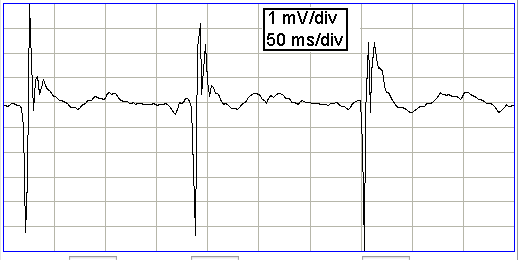
The following figure shows spikes the signal recorded by Children's Hospital Boston from epileptic rats. These spikes are larger than the spindles, and they asymmetric. They spike down in the negative direction, but barely at all in the positive. These spikes occur when the animal is having a seizure. In these animals, the seizures were the result of impact damage to the cortex.
 |
 |
 |
These seizure spikes are consistent with the coherent excitation of pyramidal neurons by another region of the cortex, as in the spindles, but without the ensuing activation that creates the symmetric spindle shape. The largest potential we observe in the spikes is of order −1.5 mV, which is consistent with our calculation for the coherent excitation of a layer of pyramidal neurons below a screw electrode. If the layer does not activate during this excitation, there will be no activation current to offset the excitory current, so that the negative excursion will be greater, and there will be no positive excursion to follow it.
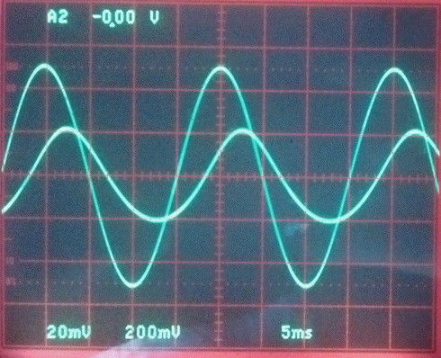
The following figure shows sustained fluctuations of 60-100 Hz in the signal recorded by the Institute of Neurology in epileptic rates. We call these fluctuations hiss. We observe hiss in rats that have been treated with tetanus toxin. Note the shorter time scale of 100 ms/div.
 |
 |
 |
The peak-to-peak amplitude of the hiss is roughly 400 μV. Such activity is consistent with excitation of a pyramidal layer by itself. Over 5 ms the excitory current builds up, followed by activation of the entire layer over another interval of 5 ms. During activation, the excitory current for the next cycle will start to build up. Thus we obtain oscillations of order 100 Hz. If we take the Fourier transform of the hiss, we see a second and third harmonic of the fundamental 100 Hz oscillation. The power of the second harmonic at 200 Hz will be in proportion to the asymmetry of the oscillation. The power of the third harmonic will be in proportion to how sharp are the edges of its extremes.
The maximum frequency of the hiss we observe is our epileptic rats is around 100 Hz. Our recordings have full sensitivity all the way up to 160 Hz. Many recent papers in neuroscience have presented what the authors believe are oscillations higher than 160 Hz in the EEG they record from human and animal subjects. The recordings they make with either skin patch electrodes, screw electrodes, or micro-electrodes. Micro-electrodes can record not only EEG, but also individual activation potentials at the same time, giving rise to a brush of high frequency power on top of a spike or trough in the EEG. So far as we can tell, however, EEG is generated entirely by post-synaptic excitory currents. These have a time constant of 10 ms. It is therefore impossible for EEG to contain oscillations much higher than 100 Hz, even if the neural network is oscillating at a much higher frequency.
Papers such as Buzski et al. show evidence of local field potentials that contain bursts of 200 Hz. But they obtained these bursts after filtering to 50-250 Hz, and their bursts of 200 Hz are always accompanied by spikes in the EEG. Any such spike will excite the 50-250 Hz filter to ring at 50 Hz and 250 Hz, so it is not clear to us that the oscillations are present in the unfiltered data. In Bragin et al., the authors report observing oscillations in EEG recorded by micro-electrodes in rats. They obtain ripples when they filter the EEG to 250-500 Hz. In their Figure 2, they show a 100-ms negative pulse in the EEG signal, with high-frequency activity near the bottom of amplitude roughly 100 μV. This suggests to that excitation is mounting in the neighborhood of the micro-electrodes, and that nearby neurons are activating, thereby generating 1-ms spikes in the extracellular potential. These spikes create a burst of high-frequency activity that stimulate a 250-500 Hz band-pass filter to produce oscillations at 250 Hz and 500 Hz. The authors appear to believe that these oscillations are present in the original signal, when in fact they could simply be an artifact of their band-pass filtering. Indeed, Benar et al. share our skepticism about the existence of high-frequency oscillations in EEG, demonstrating in a variety of ways that filtering can create the illusion that such oscillations exist.
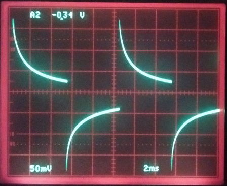
The following extracellular field potential was recorded from the dentate gyrus of a rat following perforant pathway stimulation, but not during the stimulation. The electrode is an insulated 75-μm steel wire cut off at the end to expose the conductor (see Norwood et al.).
In Andersen et al., the authors describe how a "perforant pathway volley", caused by electrical stimulation of the perforant pathway in the entorhinal area, generates sharp, short-lived, negative spikes of up to 10 mV in the extracellular fluid at the same depth as the granule cell somata in the dentate gyrus. The authors argue that the initial negative spike is due to circulating, excitory post-synaptic current, while the termination of the spike is due to circulating inhibitory post-synaptic current. As we have seen, however, excitory post-synaptic current flowing out of the somata will cause a negative pulse in extracellular potential at the depth of the somata. Conversely, if inhibitory current flowed into the somata, this would require a negative pulse. The pulses observed above are due to the circulation of activation current when an entire population of granule cells fire at once in response to a perforant pathway volley. The activation propagates up the dendrites from the somata, which causes current to flow out through the dendrite membranes, through the extracellular fluid, and back to the somata. Thus we have a negative spike on the extracellular field potential in the layer containing the granule somata, and a smaller, positive spike at the tips of the dendrites. In our section on excitory current we used the equation we derived for dipole potential to predict that an entire layer of pyramidal neurons activating within 100 μs would generate a positive pulse at the brain surface of order 15 mV. The same equation predicts a negative pulse in the layer of the pyramidal somata. Here we see simultaneous firing creates a negative pulse of 10 mV in the somata layer.
[11-APR-25] During a spreading depolarization (SD), we see a negative potential in the affected tissue when compared to the potential in tissue outside the depolarized region. The figure below shows a general seizure recorded at four locations in the brain of a mouse using one of our four-channel head-mounting transmitter.
As we show in Step Response of Metal Electrodes, stainless steel electrodes provide a clean, quiet recording, at the cost of a reduced amplitude for very low frequencies. A 8-mVpp amplitude recorded with 316SS corresponds to a 16-mVpp amplitude recorded with AgCl electrodes. We will use 16 mVpp as our assumed SD amplitude.
Under normal circumstances, living brain tissue has resistivity of order 3 Ωm. Our earlier electrode impedance calculations shows that the resistance between two screw electrodes will be of order 1.6 kΩ. In order to generate a potential difference of 16 mV between two screw electrodes across normal living brain tissue, the brain would have to provide a current of 16μA for the entire duration of the SD. It takes of order 1000 simultaneous neuron depolarizations to produ 16 μA (see Activation Current) for 2 ms. To sustain this current, we need to recruit half a million neurons per second. The more neurons that are recruited, the higher the SD potential would be.
But we see no indication that the SD potential is dependent upon the number of neurons recruited. Reports of SD amplitude as great as 30 mVpp exist, but not higher. And SD amplitudes can be as small as 3 mVpp, but not lower. The consistency in the amplitude of SD from mouse to human brains suggests that the amplitude is not a function of the number of neurons, but rather of the process of depolarization itself.
Another feature of SD is the color of the brain turning from pink to white. Blood flow slows to a stop in the SD region. The extracellular fluid is sucked into the cells, leaving the extracellular medium to act as an insulator. When the neurons depolarize, the potential difference accross the cell membranes drops to zero. The potential of the extracellular region drops and that of the intracellular region rises. We see the extracellular potential dropping by 30 mV, which is roughly one third the original difference before depolarization. This 30 mV drop creates a potential difference between the depolared and polarized regions of the brain, and current must flow between the regions. But the resitance between these two regions has been increased dramatically by the absence extracellular fluid in the depolarized region. Supposing that the resistivity increases by a factor of one thousand, the current required to maintain the SD potential would be of order 160 nA.
Our best guess is that the SD potential is provided by activation charge transfer and prolonged by the high resistivity of the brain tissue when the neurons absorb the extracellular fluid.
The EEG signal is generated by currents circulating in layers of pyramidal neurons of the cortex. When tens of thousands of such neurons act coherently, they can generate signals of several millivolts. A symmetric fluctuation of 1 mV with frequency 10 Hz is consistent with coherent excitation of one cortical region by another. A sequence of −1 mV spikes with frequency 10 Hz is consistent with the failure of the local neurons to activate after repeated excitation from another cortical region. Hiss of amplitude 400 μV and frequency 100 Hz is consistent with a cortical region exciting itself.
When a layer of pyramidal neurons is not acting coherently, we still expect its excitory current will not be zero, so our baseline EEG signal will consist of fluctuations in the baseline excitory current. What we observe in EEG is a baseline signal of order 30 μV, which suggests that the fluctuations in excitory current during periods of little activity are of order 2% of the maximum excitory current during fully-coherent excitation.
Any oscillation contained in EEG will be suppressed by the time-constant of the post-synaptic excitation process. This time constant is of order 10 ms. Even if a network of neurons were oscillating at 500 Hz, this oscillation would not appear in the EEG signal. The highest frequency oscillation we can expect in EEG will be of order 100 Hz. Our automated event detection can find high frequency oscillations easily. In thousands of hours of EEG we have examined by eye and hundreds of thousands we have been through with automated detection, we have never seen an oscillation higher than 120 Hz. So far as we can tell, there exists no mechanism by which an EEG oscillation higher than 200 Hz could take place, neither in a group of neurons acting coherently, nor in a single neuron acting alone. Reports of high frequency oscillations (HFOs) at 500 Hz are, we claim, artifacts of band-pass filtering, or individual activation currents detected by a high-impedance electrode, or they are added to the EEG by distortion in the recording system.
If our investigation has overlooked one or more sources of the EEG signal, we can expect to observe signals in our EEG recordings that are inconsistent with the sources that we have identified. Until then, however, we will trust in the accuracy of our analysis.
Screw electrodes are suitable for recording EEG. Smaller electrodes will detect EEG also, and perhaps the activation of individual neurons, although these activations will produce signals of only a few tens of microvolts. In practice, we find that a bare wire held in place with a screw is more practical and picks up a stronger signal. Because the wire is not connected to the screw, we can turn the screw to fasten it in place without twisting the wire. The wire itself can protrude a little farther down form the skull, where the EEG signal has greater amplitude.