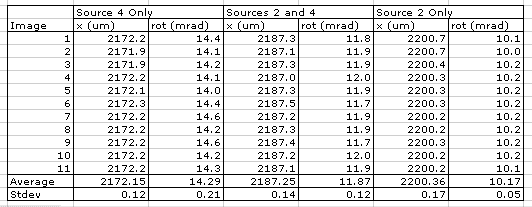
Device Mounting: Use a torque wrench to tighten the WPS mounting screw. Do not exceed torque 0.17 Nm (24 in-oz) or you may damage the kinematic mounting surfaces and ruin the absolute calibration of the instrument.
Data Acquisition: Starting with LWDAQ 7.6, the WPS Instrument acquires both WPS camera images and displays them like this. To use the new software with the WPS1, be sure to set daq_simultaneous to 0, because the WPS1 electronics do not support the use of one flash for both cameras. Also, set daq_source_device_element to 2. The result string produced by this new instrument is not compatible with software that calls the previous single-image instrument. The new result string produces eight numbers, a position and rotation for each of the four edges in the two camera images.
A Wire Position Sensor contains two cameras that take pictures of the same section of the same stretched wire from two different angles. Calibration of each camera allows us to determine for each image a plane that contains the center-line of the wire. By intersecting these two planes, we obtain the center-line itself. Thus each camera produces a plane, and each pair of cameras produces a line. We call these planes wire planes, and their intersections are wire lines.

What we call WPS1 is our Wire Position Sensor Version One, which follows our bench-top breadboard Wire Position Sensor Version Zero, or WPS0. When we present results, you can always refer to the raw tables of measurements by downloading our Excel spreadsheet here.
Here are our machine shop drawings of the WPS1 bottom plate and side plate. All dimensions are in inches.
Underside of Base Plate: Mechanical drawing of underside of Base Plate. Refers to Detail A, which you will find in the Side View.
Top Side of Base Plate: Mechanical drawing of top side of Base Plate.
Side Plate: Mechanical drawing of side plate. Includes Detail A referred to in Bottom View.
Lens Holder: Lens holder with precision pinhole, lens, and threaded light baffle.
Lens: The 9-mm focal length lens.
Cover: Mechanical drawing of cover.
Geometry: End view of WPS1 optical and mechanical geometry.
Mounting Plate Drawing: Mechanical drawing of kinematic mounting plate, shown without mounting balls.
Electronics: Manual for the WPS1 Head (A2051W), a modified version of the Polar BCAM Head (A2051L).
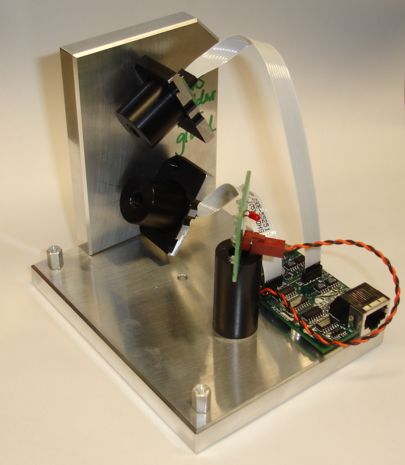
The WPS1 consists of a vertical side plate that holds two cameras, a base plate that mounts kinematically on three balls, an array of infra-red LEDs, and a cover that provides a white background for the camera images.
On the bottom side of the base plate is a kinematic mount identical to the one on the base of a BCAM, and shown in drawings such as this. The kinematic mount on the underside of the base plate consists of a cone, slot, and a flat depression. These depressions sit on three balls on a mounting plate. We provide a drawing of the mounting plate with a link above. The drawing does not show the three 0.250-inch diameter balls that must be glued into the conical depressions to complete the mounting plate. For a photograph of a mounting plate with its balls in place, see here.
A WPS mount defines mount coordinates in exactly the same way as we do for BCAMs, as we describe in the BCAM User Manual. The cone ball is the origin. The z axis points roughly in the direction of the arrow made by the three balls, but is more precisely defined by the line between the slot and cone balls. The y axis points up from the cone ball to complete a right-handed coordinate system. The WPS output is the center-line of a wire in mount coordinates. We define this line with a point and a vector. For convenience, we may pick the point on the line where it intersects the plane z=0. But the WPS1 is more accurate at z=−5 mm, so we prefer to pick the point where the line crosses z=−5 mm when we work with WPS1s. It is up to the surveyor of the kinematic mounting balls to translate the WPS measurement into a global coordinate system.
The WPS1 optical system consists of two cameras, a distributed infra-red light source, and a background screen. The cameras use the TC255P black-and-wide CCD (charge-coupled device) image sensor from Texas Instruments. We drive the cameras with an adapted version of the Polar BCAM Head (A2051L). The infra-red light source is a Nine-LED Array (A2041). The screen is a white piece of paper or a white matt-finish sticker.
To acquire images from the WPS1 cameras and flash the light source, we use the LWDAQ, a general-purpose TCPIP-based data acquisition system. The LWDAQ software is free and available here. The software provides a WPS instrument for use with the WPS1. The hardware you can buy from Open Source Instruments.
The LWDAQ creates eight-bit digitized images when it reads the TC255P through the A2051L. The WPS1 wire images, which are the basis of its wire-monitoring, are therefore eight-bit black-and-white images.
When we put a WPS in place, we mount it next to a wire without its cover. We tighten the single M4 mounting screw with a torque screw driver to 0.17 Nm torque (24 ounce-inches). We use part number 7022A611 from McMaster with a phillips head insert, part number 5751A68. You can buy the torque screwdriver form Open Source Instruments if you likel, part number TQSD-24OZ. If you tighten the screw to more than 0.17 Nm, you will drive the flat ball into the flat impression beneath the WPS base, thus ruining our 5-μm absolute calibration. If you do not secure the WPS with the screw, the cable is likely to tilt the instrument on its mount.
With the WPS secured in place, we slide the cover onto the instrument from above or from the side, taking care not to touch the wires with the folded bottom edge of the cover. If you want to make measurements without the cover, you must provide the instrument with a white background screen like the one on the inside of the cover. You can put a piece of white card next to the instrument if you like, or do something like this.
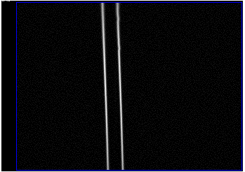
[18-OCT-07] Our images are eight-bit gray-scale arrays obtained from solid state images sensors. The aim of image analysis is to take an image like the one below and fit straight lines to the left and right edges of the wire. To this end, we began with our spot-finding routines, which we use to analyze BCAM images, as described here. We added routines that fit a straight line to the pixels in a spot. You will find our source code here. The routine that fits vertical straight lines to a spot is spot_vertical_line.

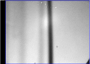
If we differentiate the intensity of this image in the horizontal direction, we obtain the following image, which we show both intensified and with its un-modified gray scale. To obtain the derivative, we let pixel (i,j) have intensity equal to that of pixel (i+1,j) in the original image minus the intensity of pixel (i-1,j) in the original image. If the difference is less than zero, we drop the sign so as to obtain the absolute value of the derivative.

The WPS analysis takes an image of a wire, obtains the horizontal derivative, and fits a line to the two white stripes in the derivative image. It displays these two lines in red on the original un-differentiated image. For a screen shot of the WPS Instrument on MacOS see here.
The spots the analysis refers to are the two collections of bright pixels in the derivative image that mark the two edges. The analysis fits lines to these two spots, even though you don't see the spots in the original image. For the meaning of other parameters, like analysis_threshold, consult the manual entry on the BCAM Instrument. In the case of the WPS, the threshold for accepting pixels into a spot applies to the derivative image, not the original image.
You can see the results of analysis printed out in the above screen shot. The position of each line is the distance in microns from the top-left corner of the image sensor to the point where the line crosses the top edge of the sensor. The rotation is the rotation of the line counter-clockwise about the vertical in milliradians. The top edge of the sensor is not the best place to obtain the position of the wire. Better is the center of the sensor. We may move the position measurement down to the center, but for now we are assuming that the routine that uses the WPS output will use the slope to determine the position of the line at the center of the sensor.
Each spot comes with an estimate of its position accuracy, which we obtain by dividing the root mean square residual from the straight line fit by the square root of the number of pixels used for the fit. In this example image, our estimate of the fitting accuracy is 0.3 μm. The WPS1 has a demagnification of 3 at the center of its field of view, so we expect the optical and electronic contribution to our position measurement error to be roughly 3 × 0.3 μm ≈ 1 μm.
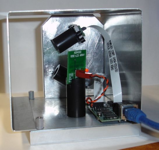
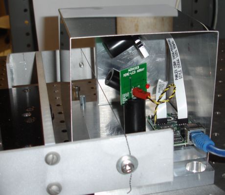
[25-OCT-07] We assemble our first prototype. Here is an End View. The two angled cameras are on the end plate. The nine-LED array is supported by a black standoff. The black tubes are the camera shields. Inside the black tubes are brass lens holders with an integrated foil aperture. The black tubes are threaded inside to eliminate internal reflections. The circuit board with an RJ-45 connector is a modified WPS Head (A2051W), which is a modified version of the Black Polar BCAM Head (A2051L). Instead of two twelve-way flex connectors, the A2051W has two eight-way connectors for the two cameras. We solder a twisted pair for the LED array.
Here is a Side View of the same prototype. This time we have a white background for the wire and a wire as well. Note how the nine-LED array is angled so that we have the nine LEDs at different heights. There will be nine dim shadows of the wire on the background instead of three strong ones.
We had to go to some lengths with a total-immersion ethanol bath to clean the CCD windows before we glued the lens holders in place. Dirt on the windows causes spots that spoil the image the derivative analysis we describe above. Below are the two images we get from the above prototype when we cover it with a box. Without the box, we sometimes see bright reflections off the wires. We can remove these bright reflections with background subtraction, as used with the BCAM Instrument.

We find that we can move the wire in a 10 mm in any direction and still obtain images as sharp as those shown above. In some directions, we can move the wire further than 10 mm. With a ruler, we measure the distance form the CCD to the wire to be 75 mm, and we know from previous measurements that the distance from the aperture to the CCD is 14 mm. We expect the magnification of our camera to be roughly 14 / 75 = 0.2. The image of a 1-mm diameter wire is roughly 200 μm on the CCD, so our magnification is indeed close to 0.2. Movement on the CCD represents movements five times larger at the wire.
The derivative analysis we describe above was erratic because the focus in our actual images is less sharp than the focus in our original image. Nevertheless, by negating the image and treating it as a BCAM spot, we obtained a resolution of order 1 μm, which we find encouraging. We are now working on a new analysis method.
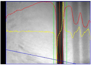
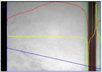
[25-OCT-07] We revived the analysis we used to fit shadows in x-ray images of ATLAS end-cap muon tubes, and applied it to the black wires in our WPS images. This analysis works by first finding the approximate wire location using the horizontal intensity profile. We obtain the horizontal intensity profile by adding all the pixels in each column together. Each column position has a total intensity, and the profile is the graph of these total intensities plotted against column number. You can see the horizontal intensity profile plotted in red on top of both images from the WPS1 below. The profile is plotted so that its maximum value touches the top of the image and its minimum touches the bottom.
After finding the approximate location of the wire, the steepest ascent fitting begins. The analysis correlates a notch pattern with the image within the green box, moving and rotating the notch to maximise the correlation. In today's version of the code, the fitting takes 1.5 seconds to complete on a 1.3 GHz laptop without the step-by-step re-display of the image (or five seconds if we re-display the images at every fitting step to show the fitting process).
When we acquire ten consecutive images from either camera, the standard deviation of the position of the image on the CCD is 0.2 μm, and of its rotation is 0.2 mrad. In terms of wire position and rotation, the standard deviation is roughly 1 μm in position (we divide by the magnification) and 0.2 mrad (the rotation on the CCD is the same as that of the wire).

The fitting analysis operates upon a rectangular area of the image, centered upon the wire. The width of this rectangle is what we call the analysis spacing. Provided that the rectangle is large enough to enclose the entire wire image, the graph above shows that our measurement of wire position and rotation is independent of the analysis spacing. For analysis spacing greater than 450 μm, the measured position and rotation vary by less than 0.1 μm and 0.1 mrad.
The wire image itself is roughly 200 μ wide, but because of its rotation of 20 mrad in the above image, the wire image spans roughly 250 pixels. The notch pattern we are using to fit with the wire image is 400 μm wide. With rotation, the pattern spans roughly 450 μm. We believe this explains why we need an analysis spacing greater than 450 μm to obtain an accurate measurement.
We could use the yellow line, which is the derivative of the horizontal intensity profile, to determine the width of the wire image. If the wire were exactly vertical, the minimum and maximum of the yellow graph would mark the left and right edges of the wire. But the wire is not exactly vertical. We will think about how we can obtain a good measurement of the wire thickness from the fitting analysis. The measurement will have to be insensitive to de-focus and rotation of the wire image.
The shadows in the images are visible in the horizontal intensity profile. If one of these shadows were to touch the wire image, we would see a large error in image position. The shadows are up to one fifth as dark as the image, and they do touch the wire image when the wire is close to the background screen. Such shadows can displace the image center by up to one tenth of the image width, or tens of microns. We must ensure that the shadows stay clear of the image. We plan to move the light sources so that they are above and below the height of the wire, and cast the wire shadow out of the field of view of the camera. In all cases, keeping the background screen at least 10 mm from the wire helps dim the shadows and keep them away from the wire.
We varied the light source flash time in order to see how sensitive the fitting analysis was to the contrast in the image. We used the following script in the Toolmaker.
for {set x 0.01} {$x <= 0.3} {set x [expr $x * 1.1]} {
  set LWDAQ_config_WPS(daq_flash_seconds) $x
  LWDAQ_print $t "$x [lrange [LWDAQ_acquire WPS] 1 2]"
}
The graph below shows the effect of varying the flash time by a factor of thirty.
The fitting analysis is insensitive to the image brightness, as you can see in the graph above. As the exposure time increases from 30 ms to 300 ms, the position varies by roughly 0.1 μm rms, and the rotation varies by roughly 0.1 mrad rms. We obtained our results with a script like the one we list above.
Given the position and rotation of a wire image in a WPS camera, we want to determine the plane that must contain the center-line of the wire. With one such plane from each of two cameras, we can determine the center-line itself by intersecting the two planes. When we work with these planes and lines, we will do so in the coordinate system of its three mounting balls, which we call mount coordinates. The geometry of each WPS1 is pretty much the same, but on the level of 100 μm and 10 mrad, the exact locations and orientations of their components vary. It is precise knowledge of the locations of its components that allows us to convert a WPS's optical measurements into the position and orientation of the actual wire. Measuring these locations and orientations is the process of calibration. The numbers specifying the locations and orientations are the calibration parameters.
We thought initially to calibrate WPS instruments with wires in precisely-known locations. We would hold wires in V-slots, measure the V-slots with our CMM, and so obtain the locations of the wires, or something like that. We considered calibrating WPS cameras with Proximity Masks. But we settled upon the use of ground steel pins.
Aside: The Proximity Mask is a variety of Rasnik Mask. Brandeis University designed the Proximity Mask, and both Brandeis University and Open Source Instruments have built Proximity Masks in quantity. The only documentation we can find on the Proximity Mask is a description of the Proximity Mask Head (A2045) and an account of an experiment called Proximity Camera Gradient. A Rasnik mask is a chessboard pattern illuminated from behind. The LWDAQ program's Rasnik Instrument is for use with Rasnik masks. We describe the Rasnik image analysis code used by the Rasnik Instrument in Rasnik Analysis. One way to calibrate a WPS is by placing a calibrated Proximity Mask in two known locations with respect to its mount. The mask will lie in the WPS's z-y plan. It will be vertical and parallel to the nominal wire direction. The WPS would obtain an image something like this.
We ordered some 1.588-mm diameter (1/16") precision-ground stainless-steel 40-mm long dowel pins. By placing such a pin in the field of view of the WPS, measuring the pin and the WPS mounting balls with a CMM, and moving either the pin or the WPS to several different positions, we believe it is possible to calibrate the WPS with absolute accuracy limited only by that of the CMM. The CMM we use is accurate to 2 μm. With four wire positions, we obtain eight measurements of position and rotation from each camera, which is sufficient to determine the camera's calibration constants. The advantage of steel pins over Rasnik masks is that it is conceptually simpler, presents the WPS with a calibration target almost identical to a wire, and can be duplicated at other laboratories more easily. We study the performance of steel pin images below.
We describe the development of our steel-pin calibration procedure in WPS1 Calibration.
[09-APR-09] We have built and calibrated a total of 8 WPS1-Bs and 4 WPS1-As to date. The WPS1-Bs absolute calibration error is between 1.3 μm and 2.5 μm. That's the error measuring wire position across the field of view, and is therefore the sum of the errors from the two cameras that determine the wire position by triangulation. The calibration error of the WPS1-As is between 4.5 μm and 13 μm.
The WPS2 optics consist of a lens, aperture, sensor, lens holder, and the baffle. We model the optics as virtual thin-lens systems, tracing rays through single-point apertures that we call the camera pivot points. The actual lens is not thin: it is 2.75 mm thick and only 6.0 mm in diameter. The aperture is not coincident with the lens center: it is a hole in a metal sheet placed behind the lens. For proof that the WPS optics are equivalent to a thin-lens system for small ray angles, see Page One and Page Two of a derivation. In the equivalent thin-lens system, straight rays pass through the pivot point. The purpose of Camera Calibration is to determine the location of the pivot point, the location of the sensor center, and the orientation of the sensor.
In Focus, we discuss the development of the WPS1-A optics, with its home-made pin-hole aperture and adaptation of existing lens holders and standoffs. In Aberration we discuss the most prominent aberrations in the WPS1-A optics. These aberrations arise because the WPS1 camera accepts rays at angles up to 150 mrad. We cannot rely upon our small-angle thin-lens approximations when a ray enters a lens at 150 mrad. The sine of 150 mrad is 0.1494, a difference of 600 μrad. In Distortion we show how the image is distorted when the camera axis is not perpendicular to the sensor.
[10-APR-08] We have made a total of four WPS1s so far, including eight hand-made, aluminum foil, pin-hole apertures. These apertures vary in diameter from 200 μm to 300 μm, which explains why some WPS1s are more sensitive to light than others. We recommend using automatic exposure adjustment to account for the different aperture diameters.
| Parameter | Value |
|---|---|
| Aperture-CCD | 9 mm |
| Pivot-CCD | 11.4 mm |
| Aperture Diameter | 250±50 μm |
| Aperture Centering | ±1 mm |
| Lens Focal Length | 9 mm |
| Lens Diameter | 6 mm |
| Focal Point of Lens to CCD | 11 mm |
| Flat of Lens to CCD | 10 mm |
| CCD Width | 3.4 mm |
| CCD Height | 2.4 mm |
| CCD Pixel Size | 10 μm × 10 μm |
| Field of View | ±150 mrad × ±100 mrad |
| Aperture Height Above End Plate | 15 mm |
| Aperture to Front of CCD Mounting Plate | 4 mm |
The aperture-ccd distance is the distance between the aluminum foil pin-hole aperture and the CCD surface. The pin-hole is just behind the knife-edge aperture of the lens holder. The WPS1-A brass lens holders are 7-mm long versions of this 5-mm lens holder. The extra 2 mm is on the far end from the lens. The total distance from the aperture to the end of the lens holder is 4 mm. We add another 3 mm thickness of the CCD mounting plate, and another 2 mm from the CCD glass surface to the CCD surface. The total aperture-ccd distance is 9 mm.
The pivot-ccd distance is the distance from the pivot point of the thin-lens equivalent camera to its sensor. Because the convex surface of the lens is 2.75 mm from the aperture, the lens acts like a magnifier for aperture-ccd distance, so that the pivot-ccd distance increases. According to our calculations, pivot-ccd and aperture-ccd are related as follows.
r' = r + γ/(1 − γ/f)
Here we have r' as pivot-ccd and r as aperture-ccd with γ as the distance from the aperture to the lens and f as the lens focal length. Inserting the WPS1-A values, we get r' = 11 mm. There is also a 0.75-mm thick window over the CCD. This window is equivalent to 1.1 mm in air, and increases r' by another 0.4 mm. Our estimate of pivot-ccd is therefore 11.4 mm. Our measurement of field of view below suggest the pivot-ccd distance is 11.4 mm. But 0ur calibration procedure suggests a value of 11.9 mm.
The aperture centering is how well we center the aperture on a line drawn perpendicular to the CCD through its center, and how well the aperture is centered upon the lens. These are two different alignments, but their variability in the WPS1-A optics are roughly the same. In theory, the poor centering of the aperture cause aberrations that in turn cause errors in our wire measurements of order twenty microns.
[12-DEC-08] After considering focus, aberration, and distortion, we design the WPS1-B optics. The new optics uses a new lens-holder to place the aperture flush up against the center of the curved surface of the lens, thus reducing aberration and distortion. A 200-μm precision steel aperture gives us more consistent depth of field.
| Parameter | Value |
|---|---|
| Aperture-CCD | 10 mm |
| Pivot-CCD | 10.4 mm |
| Aperture Diameter | 200±5 μm |
| Aperture Centering | ±100 μm |
| Lens Focal Length | 9 mm |
| Lens Diameter | 6 mm |
| Focal Point of Lens to CCD | 11 mm |
| Flat of Lens to CCD | 12 mm |
| CCD Width | 3.4 mm |
| CCD Height | 2.4 mm |
| CCD Pixel Size | 10 μm × 10 μm |
| Field of View | ±160 mrad × ±110 mrad |
| Aperture Height Above End Plate | 15 mm |
| Aperture to Front of CCD Mounting Plate | 5 mm |
The lens holder centers the aperture to within ±50 μm with respect to the lens and the image sensor, thus reducing aberration and distortion by a factor of ten. The combined lens holder and camera shield greatly simplifies assembly of the WPS1. The aperture in a steel disk 9.5 mm in diameter and 125 μm thick with the hole centered to better than 50 μm. Each aperture costs around $30 from Edmund Optics. In the new optics, with the curved surface of the lens facing the image sensor, we move the aperture and lens 1 mm farther from the CCD so that we keep the lens-CCD distance at 11 mm.
The focal range of the camera remains 50 mm. Even though the aperture-ccd distance has increased, the pivot-ccd distance decreases. The convex surface of the lens is now flush up against the aperture. The value of γ in the equation above drops to zero. We still have the CCD window, so with its effect added to aperture-ccd, we expect pivot-ccd to be 10.4 mm. The field of view increases slightly compared to the WPS1-A.
As we report in Calibration, the WPS1-B optics are accurate to 1 μm in its field of view, and the WPS1-A optics are accurate to only 3 μm. The resulting WPS1-B overall accuracy when we combine the measurements of the two cameras to determine wire position is 3 μm, while that of the WPS1-A is 7 μm.
[16-APR-10] The WPS1-B has trouble viewing the white Vectran wire favored by CERN. This wire is manufactured by a company called Vectran, and is made of sound vectran fibers. We find that the WPS1-A, with its slightly larger aperture, is able to obtain clear images of this same wire. We also note that the WPS1-B optics provide greater depth of field and sharper focus than is necessary.
[04-MAY-10] We introduce the WPS1-C, which is identical to the WPS1-B except it uses a 300-μm aperture instead of a 200-μm aperture. We have 3 WPS1-C devices assembled and ready to calibrate. We obtain sharp images within and beyond the dynamic range of the device. Saturation of the image sensor with light occurs above exposure times of around 0.4 s, compared to the WPS1-B's saturation time of around 900 ms.
[13-MAY-10] We calibrate all three WPS1-C with our existing CMM-based calibration procedure and obtain calibration accuracy between 1 μm and 2 μm. The WPS1-C, with its larger aperture, provides better performance with the white vectran wire than the WPS1-B. Nevertheless, performance is still limited by the brightness of the image compared to the electronic noise. We decide to dismantle Q0129, a WPS1-A, and replace its foil apertures with precision 500-μm apertures and so produce the WPS1-D. We order the required parts.
[09-FEB-11] We rebuild Q0129 as a WPS1-D with 500-μm apertures. We calibrate it. The calibration error is 2.3 μm. The images are bright and sharp at all ranges. This device's cameras can obtain fine images of a white Vectran wire with exposure time 200 ms, and of a blackened wire with exposure time 50 ms.
The WPS1 lens and aperture must provide adequately sharp images of wires across the dynamic range of the instrument. The dynamic range is the intersection of the two camera fields of view, as shown here. We prefer our derivative analysis to our fitting analysis, so we would like our wire images to be sharp over the dynamic range. Sharper images favor the derivative analysis, as we discovered below. We concluded that the requirement that we be able to analyze an image of a Rasnik mask with 340-μm squares is adequate to ensure that we can use our derivative analysis over the entire field of view, so we proceed with Rasnik masks as a test of image sharpness.
In both calibration positions of the mask, the mask image must be sharp enough for the rasnik analysis. This puts constraints upon the camera optics, which we discuss in Rasnik Depth of Field.
If the dynamic range of the WPS1 is ±5 mm in x, we might place the mask at ±2.5 mm and require that it be in focus at these two positions. As we show in Rasnik Depth of Field, a Rasnik designed for maximum depth of field obeys:
D = 4λc/πs,where D is the aperture diameter, λ is the light wavelength, c is the pivot-ccd range, and s is the maks square size. If we use s = 340 μm (these are the largest squares we have available), λ = 875 nm (the WPS1 infra-red LEDs), and c = 12 mm (as applies to the WPS1), we obtain D = 40 μm. The largest tolerable deviation, a, in pivot-ccd will then be:
a = πs2/4λ = 100 mm.What we see here is that a diffraction-limited camera has tremendous dynamic range, but at the same time has such a small aperture as to be incapable of gathering enough light.
Our first WPS1-A uses a lens-to-ccd distance of roughly 14 mm, and a lens of focal length 9 mm. The focal range is 1/(1/9 − 1/14) = 25 mm. The intersection of the two camera field of views is at roughly 50 mm, at twice the focal range. Because they are out of focus, the images are not sharp enough for our originally-planned derivative analysis, but they are fine for our fitting analysis.
We made the aperture of the first WPS1-A by gluing aluminum foil behind the lens in a 10-mm BCAM lens holder (the one in the drawing is only 5 mm long) and puncturing the foil behind the center of the lens with a sewing pin. The hole is approximately 300 μm in diameter. We tried a smaller hole made with piano wire, but the images it provided were too dark.
The lens-to-ccd distance is not the same as the pivot-ccd distance. The virtual camera with which we model the WPS1 camera ignores aperture width and defocus. The pivot point is very close to the center of the aperture. The lens-to-ccd distance is the distance from the effective focal point of the lens to the image sensing surface. Our lens is the NT32-469 from Edmund Optics. Its effective focal point is 1 mm in front of its flat surface. Its effective focal length is 9 mm. We have the flat surface facing the aperture and mounted 2 mm from the front of the lens holder. The effective focal point is 1 mm from the front of the lens holder. The lens holder is 10 mm long. The hole in the plate that holds the image sensor is 3 mm deep before we come to the window of the sensor. The image sensor is 2 mm below the top of the glass. The lens-to-ccd distance is 14 mm.
With the wire at range 50 mm, our 9-mm lens makes a sharp image 11 mm from it's effective focal point, or 3 mm in front of the image sensor. The image on the sensor will be blurred by 3/11 of the aperture diameter, or 80 μm. This is indeed what we see in initial WPS1 images. In the plane of the object, this blurring is 50/14 times larger, or 300 μm. The maximum tolerable blurring of a Rasnik Mask is half a square width. With 340-μm squares, we can tolerate 170 μm of blurring, but not 300 μm.
[09-NOV-07] We conclude that the existing WPS1-A optics are not able to view Rasnik masks during calibration because the focal range is only half the operating range. We will improve the image quality by shaving 3 mm off the lens holder and reducing the pivot-ccd range to 11 mm. Now the focal range will be 1/(1/9 − 1/11) = 50 mm, right where we want it, and the blurring ±3 mm on either side of the focal range will be only 10 μm. The Rasnik image will be sharp. So will the wire images. We might be able to return to the faster derivative analysis. The fitting analysis will be more accurate.
We could use the 2-mm diameter aperture built into the BCAM lens holder instead of a pinhole in foil. With a 2-mm aperture and the lens-to-ccd distance reduced to 11 mm, the blurring ±3 mm on either side of the focal range would be only 175 μm, half of what we see now. With the built-in aperture, we can expect it to be centered upon the lens holder to better than 100 μm. The optical assembly more precise. We would also obtain brighter images. The 175 μm blurring at our limit of 170 μm for blurring of a 340-μm square. We will have to try the built-in aperture with a Rasnik mask and see how it performs.
[14-NOV-07] We cut 3 mm off the back of each lens holder. Our aperture is still ≈300 μm. We placed a rasnik mask with 340-μm squares in front of one of the new cameras and took images at various ranges. We found the range over which we could analyze the resulting images was limited by the size of the squares in the image, not by blurring. We observe no blurring from range 25 mm to 70 mm.
The Rasnik analysis provides us with an estimate of our error in measuring mask position. We tabulate this error estimate with range below, as well as the field of view.
| Lens-Mask Range (mm) | Rasnik Error (μm) | Field of View (mm) |
|---|---|---|
| 15 | 2.8 | 4 |
| 25 | 2.1 | 7 |
| 35 | 1.3 | 10 |
| 45 | 1.4 | 13 |
| 55 | 1.9 | 16 |
| 65 | 2.0 | 18 |
| 75 | 2.3 | 21 |
| 85 | 2.9 | 24 |
| 95 | 2.2 | 27 |
A lens-to-ccd distance of 11 mm combined with an aperture of 300 μm will give us sharp images, excellent depth of field, enough light, and allow us to use our derivative analysis and calibrate the sensor with rasnik masks. We use these dimensions in the WPS1-A. We do our best to make a 300-μm aperture with a pin. We find that the optimum exposure time for a WPS1-A image is between 50 ms and 100 ms.
In the WPS1-B, we switch to a 200-μm precision aperture. The smaller aperture requires an exposure time between 100 ms and 200 ms, which is twice that of the WPS1-A. But the cameras are in focus from a range of 15 mm, just outside the light baffle of the lens holder, to 100 mm, right up against the lid. When we remove the lid, we can take clear pictures of faces and over-head lights in the laboratory. The depth of field appears to extend to infinity.
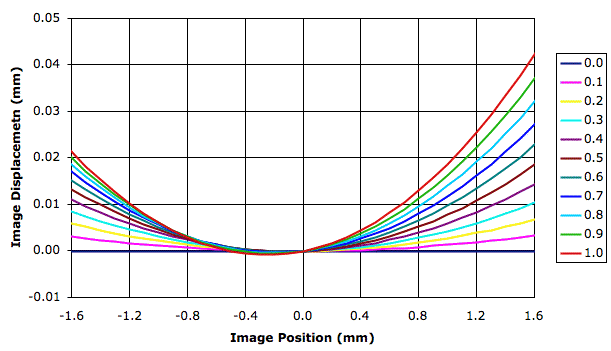
[10-APR-19] As we describe in elsewhere, our calibration procedure revealed that our pin-hole camera model of the WPS1-A optics provided only 20-μm accuracy over the field of view. Images on the CCD appear to be displaced from their correct locations by several microns. The WPS1 aperture is only 250 μm in diameter. If this aperture is centered perfectly upon the lens, neither spherical aberration nor coma aberration can account for image displacements of several microns. Let us consider the effect of the aperture being offset from the center of the lens.
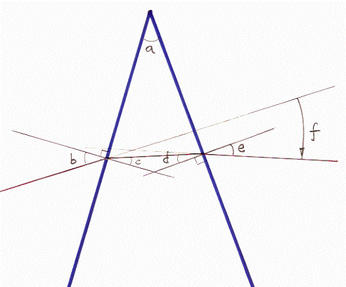
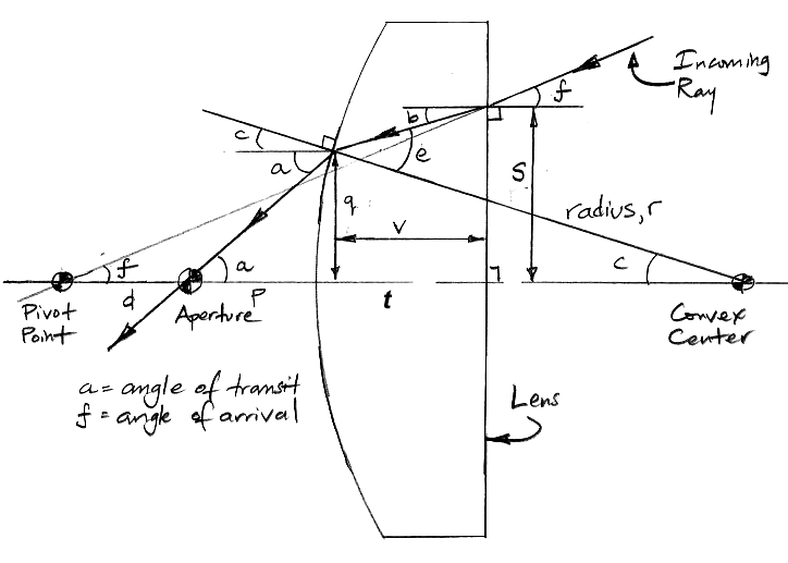
In the above figure, a ray enters a glass wedge with angle of incidence b and leaves with angle of refraction e. The internal angle of the glass wedge is a. The net change in the ray direction is angle f. Our pin-hole camera model of the WPS1 optics assumes that the angle f is linear with b. The following graph shows the non-linearity in f as it varies with b for glass with refractive index 1.5 and various wedge angles.
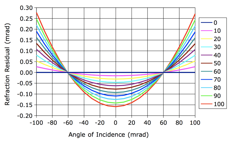
The wedge angle of a lens is zero at the optical center of a lens, but the optical center can be offset from the physical center. The wedge angle of our 32469 lens at its physical center is ±1.5 mrad. When we punch a hole in the aperture foil with a pin, the hole can be off-center by 500 μm. Our lens has a convex radius of 6 mm, so a 500-μm offset means the wedge angle in front of our aperture can be as large as 80 mrad. The optical center of the lens is far closer to the physical center than is our aperture. If we look at the a = 50 mrad graph above, we see that a ray entering at −100 mrad will deviate from the direction predicted by our thin-lens, pin-hole camera model by 0.2 mrad. This 0.2 mrad will change the apparent position of a wire 50 mm away by 10 μm.
Our best pin-hole camera approximation of the WPS1-A is inaccurate by roughly 20 μm rms in the field of view, as we show here. It may be that the greater part of these errors is due to poor centering of the aperture upon the lens. The WPS1-B optics centering of the aperture and lens to better than 200 μm. The wedge angle in the WPS1-B will be at most 30 mrad, aberration will be less than 80 μrad, or 4 μm at range 50 mm. Taken over the entire field of view, the rms error should be less than 2 μm.
Another source of aberration is the displacement of the aperture from the center of the lens. The WPS1-A aperture is 1 mm from the flat side of the lens. The effective focal point of the 32469 lens is 1.0 mm from the flat side, a total of 2.0 mm from our aperture. Rays that pass through the aperture at an angle to the optical axis will use a different portion of the convex surface than rays that are parallel to the optical axis. The following diagram shows a ray entering the convex side of the lens, exited the flat side of the lens, and passing through the aperture at a transit angle a.

In our virtual thin-lens model of the WPS1-A optics, the pivot point is the point on the optical axis through which all incoming rays intersect before proceeding to the image sensor. The program pivot.pas takes the aperture center as its coordinate origin and places the flat side of the lens a distance p along the x-axis. It varies the transit angle, a, made by a ray passing through the aperture, and determines where and in which direction the ray passed through the convex surface of the lens. It extrapolates this incoming ray to the optical axis to determine the x-coordinate of the pivot point for rays with transit angle a.
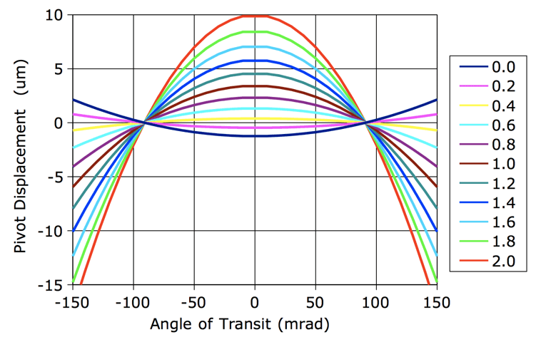
The WPS1-A and WPS2-C have p = 1.0 mm. The pivot point moves away from the lens by 10 μm as an object moves from the center to the edge of the field of view. At an object range of 50 mm, this 10 μm decreases the magnification of the camera by 0.02%. A 5-mm wire movement at the edge of the field of view will appear 1 μm smaller than a 5-mm movement at the center of the field of view. As we increase the angle of transit, the angle of arrival, e+c, increases also. Our thin-lens model assumes that the angle of arrival is linear with the angle of transit. Using pivot.pas again, we obtain the angle of arrival versus angle of transit for various aperture locations, fit straight lines, and plot the residuals.
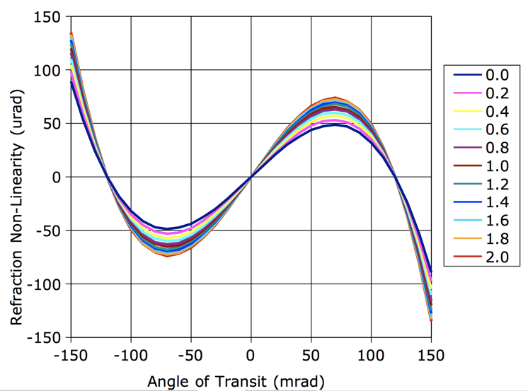
The non-linearity is the cubic term neglected by the approximation sin(θ) = θ used by the thin-lens model of refraction at spherical surface. Aperture location has little effect upon its magnitude. At the extreme edges of our field of view, for p = 1.0 mm, the non-linearity is ±100 μrad. When multiplied by a 50-mm range to wire, the wire will appear displaced by 5 μm. The rms non-linearity is 50 μrad, leading us to expect a 2.5 μm rms error in the field of view.
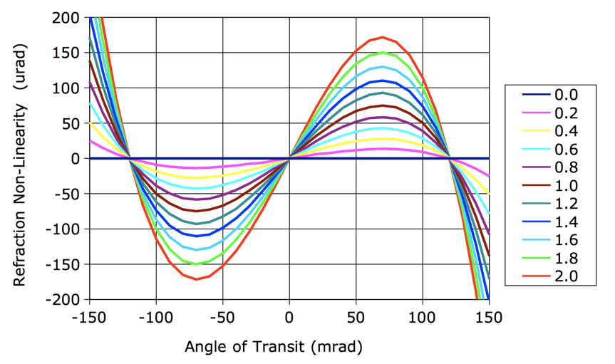
We now use pivot.pas to combine these two aberrations and calculate the nonlinearity in our measurement of the movement of an object at range 50 mm. We find that the two aberrations combine to create an aberration of twice the size. We fit a straight line to object position versus the tangent of the transit angle, and plot the residuals to this fit as our measurement of non-linearity in object position measurement.

The above cubic non-linearity appears to be robust in the face of small movements of the aperture. We could, in principle, correct this aberration with one cubic correction term added to our WPS camera parameters, without even measuring the correction during calibration. Having performed this calculation while making WPS1 sensors, however, we thereafter flipped the lens so that its convex side would be close to the aperture. We believed this would reduce both the wedge angle error and the aperture-displacement error. The WPS1-B lens holder places a 200-μm aperture 400 μm from the center of the convex surface of the lens. The WPS2-B lens holder places a 500-μm aperture 400-μm from the surface. The following diagram shows a ray arriving at the flat side of the lens and existing through the convex side before transiting the aperture.
We use program pivot_reversed to determine the nonlinearity of the angle arrival with respect to the angle of transit.
The WPS1-B and WPS2-A use this reversed-lens arrangement, as shown here, in which the center of the aperture is approximately 400 μm from the convex surface of the lens. We expect the refraction nonlinearity to be 25 μrad rms across the field of view, which is half the non-linearity we observe with the flat side of the lens facing the aperture. But if the aperture were to end up 1 mm from the lens, the non-linearity increases to 65 μrad rms, and at 1.4 mm to 100 μrad rms. With the flat side of the lens facing the aperture, the non-linearity is only weakly affected by the exact aperture location.
We use the same program to calculate the position of the pivot point versus angle of transit for various aperture positions. When the aperture is flush up against the lens, the pivot point is 920 μm into the glass. When the aperture is 1 mm from the lens, the pivot point is 170 μm in front of the glass. It is not the exact location of the pivot point that concerns us, but the displacement of the pivot point with angle of transit.
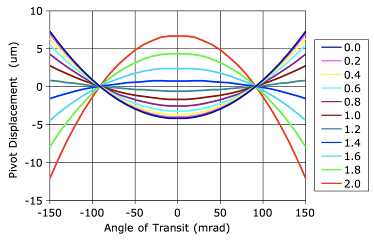
When the aperture is 0.4 mm from the lens, the pivot point of our virtual thin-lens system will move 10 μm towards the lens as an object moves from the center of the field of view to the edge. For object range 50-mm, the magnification of the image will increase by 0.02% at the edge of the field of view. A 5-mm movement at range 50 mm on the edge of the field of view will appear 1 μm larger than a 5-mm movement at the center of the field of view.
We now use pivot.pas to combine these two aberrations and calculate the nonlinearity in our measurement of the movement of an object at range 50 mm. We find that the two aberrations cancel to create a far smaller net aberration. We fit a straight line to object position versus the tangent of the transit angle, and plot the residuals to this fit as our measurement of non-linearity in object position measurement.

For the WPS1-A, WPS2-A, and WPS2-B, we use the plot for p = 0.4 mm, which predicts a maximum aberration of 5 μm at the edges of the field of view, and rms nonlinearity 2 μm.
The image sensor (the CCD) has its own axis: the line perpendicular to its surface that passes through its center. The camera axis, meanwhile, is the line passing through the center of the aperture and the center of the sensor. We can simplify our camera calibration if we assume our sensor axis is coincident with the camera axis. We make this assumption for the BCAM. Suppose we make this assumption for the WPS1-A. Images on the sensor will be displaced by the fact that the actual sensor axis is not coincident with the camera axis, as shown in the following diagram.
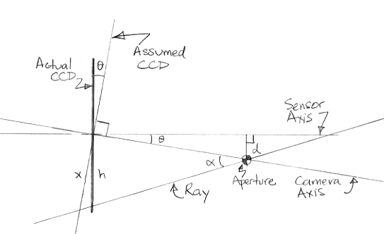
The aperture is offset by a distance d from the sensor axis. If the sensor were perpendicular to the camera axis, the ray would hit the surface at a distance h from the center. But because of the angle θ between the camera and sensor axes, the ray crosses at distance x from the center. The distortion of our image is the distance x-h.
The WPS1-A optics center the aperture to within ±1 mm. Even if the aperture is only 300 μm off-center, we will see distortion of 10 μm at the sensor edges. If we are measuring the position of a wire 50 mm away at the edge of the field of view, our error will be roughly 50 μm. We conclude that we cannot assume that the WPS1-A sensor is perpendicular to the camera axis and hope to calibrate the sensor with 5-μm accuracy. Nevertheless, we were able to calibrate a WPS1-A with the perpendicular assumption and 5 μm rms calibration error, as we show here.
In the case of the BCAM, the lens-ccd distance is 75 mm and the centering is ±500 μm. Our program tells us the distortion on the BCAM sensor will be less than 0.3 μm, which is less than the BCAM's advertised 0.5-μm accuracy in image location across the sensor. The dominant source of this distortion in the BCAM is not the displacement of the aperture, but rotation of the image sensor by θ when mounting.
The WPS1-B lens holder centers the aperture to ±125 μm with a lens-ccd distance of 10 mm. Our program tells us the distortion on the sensor will be 3 μm at the edges of the field of view, which implies a 15 μm error in measurement of the position of a wire at range 50 mm. This potential error is why our WPS calibration does not assume that θ = 0. We calibrate the rotation of the CCD about all three coordinate axes.
The ideal illumination of the screen behind the wire would be bright and uniform. Non-uniformity in the background intensity causes an apparent shift in the wire position. A shadow cast by the wire is an example of a sharp variation in background illumination. The ideal illumination must therefore avoid creating shadows in the field of view.
Another potential source of error is reflection of light off the wire to the camera. We avoided bright reflections in the WPS1 by placing the source of light aside from the camera along the length of the wire. The displacement of the light sources along the wire avoids direct reflection off the wire surface into the camera. But we still see signs of light scattering off the wire, which makes the sides of the wire appear brighter than they would if the only source of light were the screen behind the wire. The ideal illumination would cast no light upon the wire, and illuminate only the background screen.

The WPS1-X uses two mirrors to direct visible red light around the back of the wire and onto the screen. Because the light does not shine directly upon the wire, there are no shadows and there is no illumination of the wire itself. We use two light sources in an effort to make the background intensity uniform for both cameras. For a photograph of our WPS1-X, see here.
Below are three images, showing how the background intensity varies as seen by Camera 2 (the upward-looking camera) when we flash the two LEDs.
The illumination provided by our two LEDs is not uniform. The red graph is the horizontal intensity profile, which we obtain by adding the intensity of every pixel in each column. We plot the profile so that the darkest point is at the bottom of the image and the brightest point is at the top. We can express the gradient of the background intensity in units of percent full scale per percent full width. A gradient of 1 would be line from the bottom left to the top right. We estimate the gradient of the profile on either side of the wire in each image by placing a ruler on the computer screen. Our estimates of the gradient are +3 for the left image, +1 for the center image, and −0.5 for the right image.
When we measure the wire image position with the three different LED combinations, we obtain the following results.
Our resolution with each illumination is below 0.2 μm, but our measured position varies by 28 μm as we vary the illumination. From gradient +3 to +1, we see a jump of +15 μm. From gradient +1 to −0.5 we see a jump of +13 μm. Our sensitivity to illumination gradient is of order +10 μm/%/%. If we want accuracy of 1 μm on the image sensor, we need the illumination gradient to be less than 0.1. Our existing gradient with both LEDs is ten times too large.
We now return to our original nine-LED illumination, but now we combine it with our improved camera orientation and sharper focus. We increase the current through our LED array, align the array with the vertical, and look at how the shadows move with wire position. We find that the shadows never touch the wire image while the wire is within the ±5-mm area marked on our drawing above. Because the angle of incidence of the light upon the wire is low, scattering of light from the wire is dim. We moved the LED array up and down by 30 mm and watched the shadows move back and forth. We measured the image position and found it to vary by 0.4 μm rms as we moved the LED array by 30 mm.
Looking at the image on the right, we see that the intensity gradient varies from +0.5 on the left to −0.5 on the right. We expect a ±5 μm error due to these gradients. In terms of wire position, we expect a ±20-μm error, or roughly 5 μm rms. We are not satisfied with this 5-μm rms error. If we are to use our fitting analysis, we must decrease the intensity gradient by another factor of four.
If you go back to our section on our Fitting Analysis, you will see that the original images we obtained with the WPS1 were severely defocused. The fitting analysis works better on defocused images. It fits a triangular notch pattern to the wire image, and finds the center of the wire more reliably if the center is marked by a minimum of intensity. As you can see in the above images, the intensity minimum no longer corresponds to the wire center. The sharply-focused wire is, to the first approximation, uniformly dark through its width. It is the edge of the wire that defines the wire position, not the darkness at the center of the wire.
We altered the WPS analysis_min_spacing_um parameter, which changes the width of the notch we use to fit the wire shadow and the width of the image area we use for the fit. We found the measured wire position varied by ±10 μm as we increased the spacing from 400 μm to 1000 μm. With the defocused wires, we observed less than ±1 μm variation in the same experiment, as we show here.
We conclude that our fitting analysis is ill-suited to our new, sharp images. But the sharp images allow us to return to our Derivative Analysis. Our derivative analysis has several advantages over the fitting analysis.
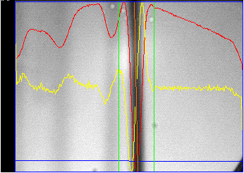
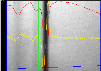
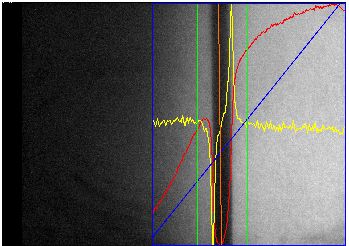
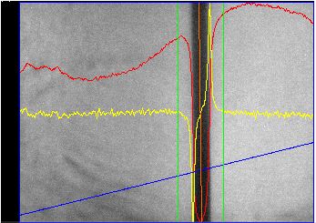
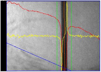
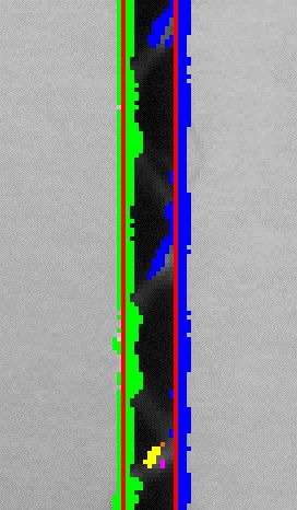
We restored our derivative-based analysis to the WPS instrument. Below you see two images taken with the screen in two different positions. The three shadows move as the screen moves. Overlaid upon the image are the horizontal intensity profile, now in green instead of red, the absolute-value derivative intensity profile, in yellow, and the two edges found by the analysis, in red. The horizontal blue line is the horizontal line that defines the location of the vertical edges. The derivative analysis returns the distance from the left side of the image to the intersection of the edge with the blue line.
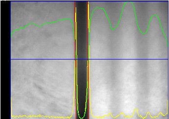
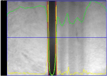
It is obvious from looking at the yellow graph that the shadows will not affect the wire unless they touch the edge of the wire. We moved the screen around and measured the edge positions. When the shadows overlap the right edge, the derivative analysis can no longer find the edge because it is no longer sharp. But so long as the shadows do not touch the image, the measured edge positions appear to be unaffected. As we moved the screen in and out, the standard deviation of edge position was 0.3 μm, and of rotation was 0.3 mrad, which is the same resolution we obtain if we leave the screen stationary.
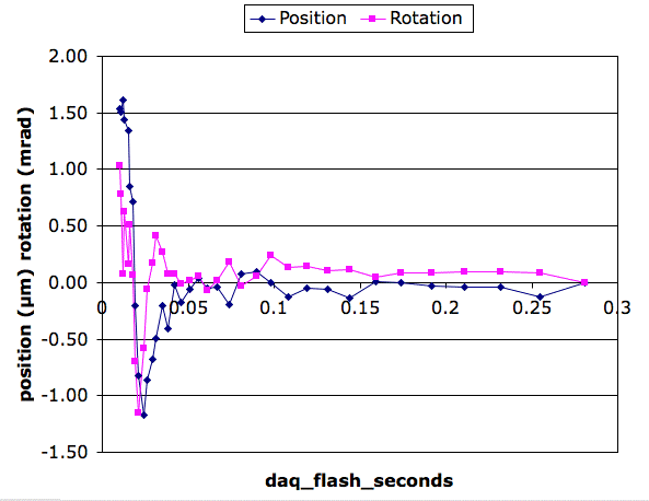
Our improved WPS optics always gives us sharp wire images. But we must still be sure that these images are bright, or else the derivative analysis will not work. We find the analysis is unreliable for an exposure time of 0.1 s, and the image begins to saturate at 0.3 s. We set the default WPS exposure time to 0.2 s. The graph below shows how the measured position and rotation of both wire edges varies with exposure time.
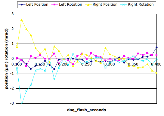
To obtain our results, we used the following script in the Toolmaker.
for {set x 0} {$x <= 0.4} {set x [expr $x + 0.01]} {
  set LWDAQ_config_WPS(daq_flash_seconds) $x
  LWDAQ_print $t \
  "[format {%.3f} $x] \
   [lrange [LWDAQ_acquire WPS] 1 2] \
   [lrange [LWDAQ_acquire WPS] 7 8]"
}
As you can see, we vary the exposure time by a factor of three and maintain resolution of 0.3 μm and 0.3 mrad.
Our derivative analysis uses a threshold to distinguish between pixels that are too dark to be part of a wire edge, and those that are bright enough. The BCAM Instrument uses a threshold to identify light spots. We discuss the effect of changing the threshold in our BCAM User Manual. We used the following Toolmaker script to vary the threshold we used with our derivative analysis when we applied it to the left image above.
for {set x 1} {$x <= 30} {set x [expr $x + 1]} {
  set LWDAQ_config_WPS(analysis_threshold) $x
  set result [LWDAQ_acquire WPS]
  LWDAQ_print $t \
  "[format {%.3f} $x] [lindex $result 1] [lindex $result 2] \
   [lindex $result 7] [lindex $result 8]"
}
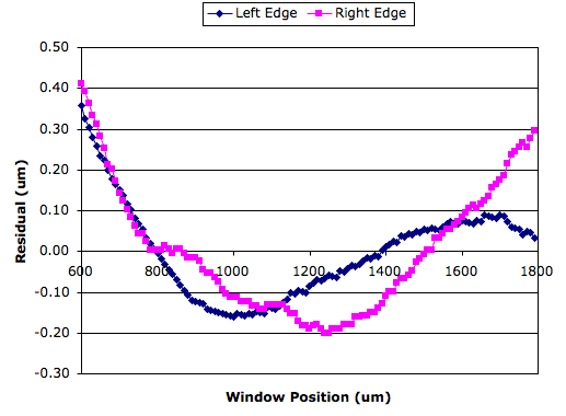
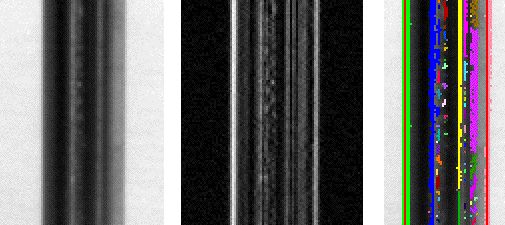
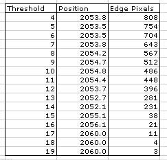
We present our results below. We plot changes in the position and rotation of each edge of our wire as a function of threshold. The maximum intensity in the derivative image is 34 counts. Our graph goes up to 20. Above 22, the plot moves off to ±10 μm.
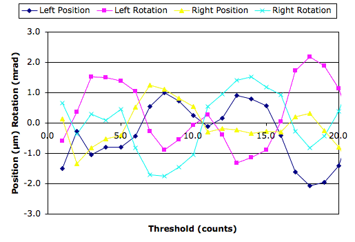
The standard deviation of position as we increase the threshold from 1 to 20 is 1 μrad, and that of rotation is 1 mrad. The WPS Instrument allows you to specify the threshold in terms of the minimum, maximum, and average intensities in the derivative image. The BCAM Instrument allows you to do the same for the original image. We obtain the best accuracy by making the threshold low, so as to include more edge pixels, and using the pixel intensity to weight its contribution to the edge. We have been using "10 #" as our threshold code, which puts the threshold 10% of the way from the average intensity in the derivative image to the maximum intensity. This gives us a threshold of 5 in the image we analyzed to obtain the above graph.
We used the "10 #" threshold code in our plot of position verses flash time. The threshold we used varied in proportion to flash time, and the measured edge positions remained stable to 0.3 μm. Our hope is that by using "10 #" we reduce the effect of threshold upon our measurements to less than 0.3 μm and 0.3 mrad.
The screen will be a white sticker on the inside of the WPS cover. Here we consider where to put the screen, and how large it must be.
The farther we place the screen behind the wires, the farther the wire shadows will be from the wires, and the less sharp the wire shadows. Our dynamic range in the vertical direction increases slightly. But the increase is not significant.With the screen father away, we get less light reflected back to the cameras. Our exposure time must increase. We find this increase does not cause us problems.
When we move the screen farther away, it must be larger. Here are four images taken with the two cameras of a ruler at two ranges. The near range is with the ruler flush up against the edge of the WPS base and standing upon our optical table. The far range is with the ruler half an inch back from the WPS base, still standing on the optical table
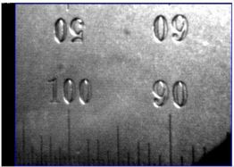
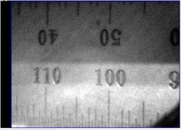
The nominal center of the WPS1 dynamic range is 50 mm up from the top surface of the 0.5-inch thick base plate. With respect to the optical table surface, the WPS1 center is 62.5 mm hight. A ruler reading of 62.5 mm Camera 1 looks down, Camera 2 looks up, as shown here.
At the near range, Camera 1 sees from 44 mm to 65 mm. At the far range, it sees from 34mm to 60 mm. Camera 2 sees from 62 mm to 83 mm at the near range, and from 67 mm to 93 mm at the far range. At the near range, the fields of view overlap by 3 mm.
Given the geometry of our cameras, as shown above, these field of view measurements imply an angular field of view in the vertical direction of 17°. In other words, the field of view subtends a 17° angle in the vertical direction at the camera pivot point. Given that the image sensor is 3.4 mm wide in the vertical direction, the 17° field of view implies that the pivot-ccd distance is 11.4 mm. In our Optics section, we concluded that the lens-to-ccd distance was 11.4 mm also.
At the far range, the fields of view are separated by 4 mm. At the near range, we need a continuous 39-mm long screen. At the far range, we can use a continuous 59-mm long screen, or two shorter screens of 26 mm each. We choose to place the screen at the far range, and use two smaller screens that do not overlap. When we set up a new WPS1, we will be able to use the screens as targets by which to orient our cameras. You will find a drawing of the cover here, but the drawing in the next section is more informative.
The cover stays in place by its own weight. The top side rests upon the top of the WPS end plate. The left side of the cover bends in at the bottom, and rests upon the top of the WPS base plate. We will put two constraining pins on the top side of the base plate to stop the cover moving to the right. The right side of the cover rests against the right side of the base plate.
With our cover designed, we arrive at our final WPS1 optical and mechanical geometry. We increase the angle between the camera axes from 60° to 62° in order to simplify our dimensions and guarantee the separation of fields of view on the inside of the cover.

The location of optical features will be accurate by construction to only ±1 mm. The mechanical parts are machined to ±0.15 mm and bent (in the case of the cover) to ±0.5 mm. In the drawing, the WPS x-direction is left, y-direction is up, and z-direction is into the page. We are looking along the wire in the direction of the arrow made by the three mounting balls. The origin of mount coordinates is the cone ball.
The WPS optical center is the center of its field of view, at the intersection of the two camera axes. The drawing shows us that the nominal x-position of the optical center is +38.0 mm. The nominal y-position is +63.2 mm. We cannot deduce the nominal z-position of the optical center from the above drawing. With a micrometer scale, we do the best we can to measure the distance from pivot point to the cone ball along the z axis on one of our WPS1-As. The nominal z-position is close to −5.0 mm.
For background screens, we will use two white long-life polyester stickers on the inside of the cover. We will leave a 2-mm gap between the stickers, centered upon the height of the WPS optical center. When we adjust the cameras during assembly, we will make sure that the inner edge of the stickers are just out of view.

The WPS field of view is a pentagon. The left edge is defined by the passage of the cover as it comes down from above to rest upon the top surface of the base plate. The remaining sides are defined by the intersection of the two camera fields of view. The field of view encloses a 10-mm square with at least 1-mm to spare on all sides. With assembly accuracy of ±1 mm, we can be sure that all WPS instruments will be able to monitor wires within the 10-mm square centered upon point (38.0, 63.2, −5). For a solid-model three-dimensional view of the WPS1 field of view, see here.
If our WPS1-As were constructed perfectly, it would have the geometry shown above. The axes of both cameras would lie in the same z-plane, with z = −5 mm. The image sensor columns would be perpendicular to this z-plane. The image sensor surfaces would be exactly perpendicular to the line joining their centers to their camera pivot points. The pivot points would be at the same x-coordinate, with x = −4.5, and separated by 50 mm. The lower camera pivot point would be at y = 37.4 mm. The Camera 1 axis would be declined at 31°, and the Camera 2 axis would be inclined at 31°. The pivots points would be 11.4 mm from the image sensors.
Our first WPS1-A lies within ±3 mm of these nominal positions, and ±3° of the nominal angles. If we assume the WPS1-A is exactly nominal, and calculate the wire position using the nominal geometry, we will arrive at a measurement of wire position that is offset by a few millimeters, scales incorrectly by a few percent, and is rotated with respect to the true coordinate system. But our estimate will nevertheless be useful in telling us when we are close or far from the WPS1-A measurement center, and it will allow us to measure the WPS precision.
We prepared an Acquisifier Script that reads both camera images and calculates the position the wire would be in if the images were recorded from a WPS with the nominal geometry. You will find the script here. The script is called WPS_1.txt. We filled it with comments so you can see how it works.
We moved our test wire in x and y, and confirmed that the sign of our measurements were correct. You can use the same script on your own WPS1 by first setting up the WPS instrument to capture an image from one or the other camera, checking that the wire is in view of both cameras, and running WPS_1.txt in the Acquisifier.
We moved the wire to the nominal center of the WPS and left it stationary. We took repeated measurements over the next few minutes. Our precision is as follows.
| Measurement | Precision |
|---|---|
| Wire Image Position (Camera 1) | 0.04 μm |
| Wire Image Position (Camera 2) | 0.12 μm |
| Wire Image Width (Camera 1) | 0.07 μm |
| Wire Image Width (Camera 2) | 0.23 μm |
| Wire Image Rotation (Camera 1) | 0.05 mrad |
| Wire Image Rotation (Camera 2) | 0.18 mrad |
| Wire Position, Horizontal | 0.52 μm |
| Wire Position, Vertical | 0.32 μm |
Our wire precision is better than 1 μm, which we are glad to see. The precision in the vertical direction is slightly better, which we expect because the cameras are more horizontal than vertical, so they are more sensitive to vertical movements.
[16-JAN-09] We now have a new WPS readout script, WPS_2.txt. This script uses camera calibration constants to transform image positions and rotations into wire positions and rotations in WPS coordinates. We include in the script the calibration constants for the default WPS1-A cameras and the calibration constants we measured and calculated for cameras Q0130 and Q0131. The user can select one of the included devices by commenting out the unused constants in the script.
[12-AUG-09] We now have an improved WPS readout script, WPS_3.txt, designed for systems with multiple devices. Camera calibration constants are stored in the text of the script itself. Each camera occupies an acquire step in the script, and post-processing in each step looks up the correct camera calibration constants using the step name. Each step is named after its camera. The result for each step is a wire plane. The result specifies the plane with the camera pivot point and a normal to the plane. The script leaves it to another program to intersect the planes for each pair of cameras and so obtain the wire line.
[25-MAY-10] A new WPS readout script, WPS_4.txt, calculates wire position for each WPS by combining the results of two acquire steps at the end of the second step.
[27-MAR-2008] So far, we have been working with wires like the Black Wire shown above. As you can see in the montage below, the black wire provides the most uniform wire silhouette. The white wire silhouette is not as dark. The tungston wire silhouette is too narrow for us to identify separate edges with our existing derivative analysis. The carbon fiber wire image shows bright spots where light reflects off the plastic braid. This image is not just a silhouette: some of our illumination is shining off features on the wire, in particular the left edge of the wire.

We would like to know how much the WPS1 measurement will be affected by movement of the wire along its axis. The carbon fiber wire has the least uniform cross-section, on account of the plastic wrapper and occasional protruding fibers. As bright spots in the carbon fiber wire image move across the field of view, without any lateral translation of the wire, we may find that we see apparent translation because of the appearance and disappearance of such bright spots from the top and bottom of the image. It is not easy to move a wire longitudinally without translating it. But we have enough information in a single image to estimate the magnitude of the error caused by non-uniformity of the wire.
The WPS analyzes the area of an image defined by its analysis bounds. The following Toolmaker script moves a 1200-μm high rectangular analysis region from top to bottom of the image in 120 steps, and calculates the wire position at each step. The change in wire position will be as if our CCD columns were half as high as it is, and we moved the wire upwards in a direction equal to its rotation with respect to our CCD columns.
upvar #0 LWDAQ_info_WPS info
upvar #0 LWDAQ_config_WPS config
set info(file_use_daq_bounds) 1
for {set mid 60} {$mid < 180} {incr mid} {
	set info(daq_image_top) [expr $mid - 60]
	set info(daq_image_bottom) [expr $mid + 60]
	set config(analysis_reference_um) [expr $mid*10]
	set result [LWDAQ_acquire WPS]
	LWDAQ_print $t "$config(analysis_reference_um) \
		[lindex $result 1] \
		[lindex $result 7]"
}
We take the measurements produced by the above script and fit straight lines to the position of both edges of the wire. We plot the residuals from the straight-line fit. A perfectly straight, perfectly-black wire should show no residual. A curving wire will show a parabolic residual. A wire with non-uniformity will show steps and oscillations in the residuals. The following graph is the one we obtain with the Black Wire.
The Black Wire performs very well. The non-uniformity error is less than 0.2 μm, and will contribute less than 1 μm to our final measurement error. We cannot say the same for the Carbon Fiber Wire.
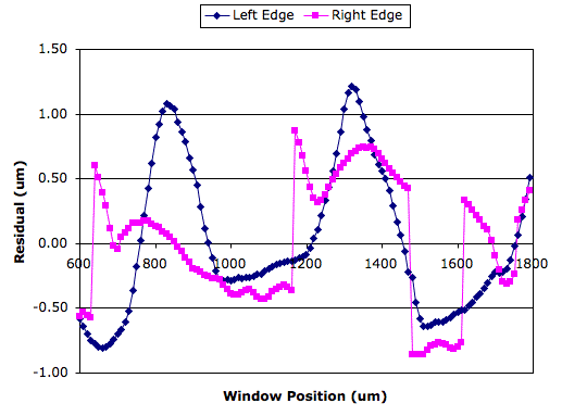
The bright spots in the Carbon Fiber Wire image cause a 0.5-μm rms error in the position of both edges, even though the brightest spots in the image are all on the left edge of the wire.
In our experiment, we use only half the CCD to obtain our measurement. When we use the entire CCD, and take the average both edge positions, we can expect the longitudinal non-uniformity error to drop to less than 0.3 μm. This error is on the image sensor. In terms of wire position, the error will roughly four times larger, or 1.2 μm. But we have two cameras, and non-uniformity errors will be independent from one camera to the next, so we expect the final wire position error to be of order 1 μm rms.
We conclude that the the wire position error resulting from longitudinal non-uniformity in the Carbon Fiber Wire image will be roughly 1 μm, which is within our calibration tolerance of ±5 μm.
[02-APR-09] We try a wire made of Vectran Fiber. We received a one-meter length of white wire from CERN. We cut it into three equal lengths and wound it together to form a single 700-μm diameter wire. We did not do a great job of winding the wire together and we can see slight variations in the wire thickness (look at the bottom two images in the montage). Nevertheless, these variations are much smaller than those we see in the carbon fiber wire, so we assume their effect upon the measured edge positions will be less than the 1 μm we estimated for the carbon fiber wire's variations.
[02-APR-09] The white vectran wire does not show up well in front of the white WPS1 background (see bottom right here). The WPS1-A, with its larger optical aperture, takes better pictures of the white wire than the WPS1-B. The original derivative analysis is unreliable in the WPS1-B with the white wire. Image noise starts to confuse the edge-finder. We added an option to the WPS Instrument whereby we can pre-smooth the image before edge-finding, using a 3×3 averaging filter. Set analysis_enable to 2 and you activate the pre-smoother. With the pre-smoother turned on, daq_flash_seconds of 0.2, and analysis_threshold of "10 #", we obtain resolution 1 μm in locating edges in the image. With daq_flash_seconds of 0.4, resolution improves to 0.5 μm.
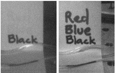
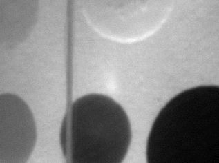
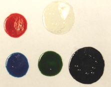
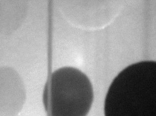
We colored the wire with red ink, hoping to make it more visible. We saw no improvement. We colored it with blue ink. Still no improvement. The next day we tried black ink. Now the wire shows up just fine. It turns out that the red and blue inks are white in the WPS1's infra-red light, as we show in the figure below.
You can see an image of a black vectran fiber on the bottom-left of the montage. The black wire shows up well. Without pre-smoothing, using daq_flash_seconds of 0.2, we obtain 0.2 μm resolution in edge-position on the image. With pre-smoothing, the resolution improves slightly to 0.15 μm. With pre-smoothing, the analysis is effective for exposure times down to 30 ms. Without pre-smoothing, the exposure time must be at least 100 ms.
[04-MAY-10] We present further development of the WPS image analysis below.
[01-JUN-10] We receive five colors of alcohol-based temporary tattoo ink from Olive Branch Skin Care and try them out in infra-red light. We place a spot of each color ink on a piece of paper and use this piece of paper as the WPS screen in both infra-red and white light.
The temporary tattoo ink dries quickly. It is not corrosive. When the ink dries, it is tacky to the touch and remains flexible. We dye a piece of white vectran wire using the black ink. We apply the black ink by wiping the wire with a sponge soaked in the ink. With the black wire we obtain good image contrast using a WPS1-B with 100-ms exposure.
[02-SEP-10] We hear from Georg Gassner of SLAC non-conducting wires can get be deflected by static charge. "We saw quite a lot of deflection due to static charge. We had two fishing (monofilament 80lbs proof) lines stretched in parallel separated by 5mm over a distance of 150m. Over time the distance between the two wires changed in the middle to about 10mm." We purchased two types of conducting ink from SEMicro. One is silver paint, SP-18. The other is carbon paint, CP. We set up two 10-cm lengths of white vectran wire and painted them with the brushes that came with the ink bottles. The carbon paint spreads around the wire more easily than the silver paint. A week later, we inspect the wires. The paint has soaked well into the fibers. It does not appear to have changed the fiber cross-section. The resistance of the fiber with silver paint is 10 Ω/cm. The silver paint dries to a dull silver gray. The resistance of the fiber with carbon paint is 1 kΩ/cm. The carbon paint dries to a matt black color.
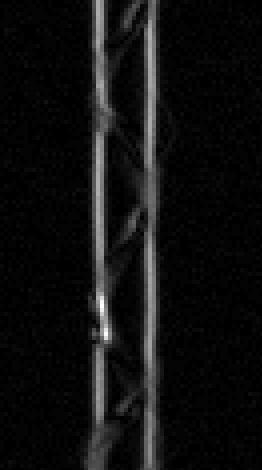
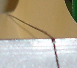
We purchased some 1/16" (1.588 mm) diameter, 1.5" (38.1 mm) long, 18-8 stainless steel, ground dowel pins, part number 90145A427 from McMaster-Carr. The diameter of these pins is accurate to ±0.0001" (2 μm) all along their length. We believe they are straight to ±2 μm as well. We fixed one such pin in front of our WPS cameras with a standoff glued to the WPS base, as shown below.

We are interested in steel pins for two reasons. They are large enough for us to measure with our CMM. They are stiff enough to withstand the CMM probe pressure without distorting. As we discuss above, steel pins and a CMM are one way of calibrating WPS instruments. Another use for steel pins is to test the inherent stability of the WPS. The pin shown above is attached to the WPS base. It will not sag or bend with temperature. Any apparent movement of the pin will be due to an error in the WPS.
The figure above shows an image of the fixed pin. We see reflections of our LEDs in the surface of the pin. The pin surface has been ground smooth. The surface has microscopic features that wrap around the circumference of its surface. These features reflect the LED light into our cameras. Up until now, we have used threshold code "10 #" to place the edge pixel threshold 10% of the way from the average to the maximum intensity in the derivative image. But when we this code with images of a steel pin, the two clusters of pixels on the right side of the image occasionally join up and move the fitted edge towards the center of the wire. When we set the threshold code to "20 #", the true edge cluster is always distinct from those associated with the reflective stripes on the wire.
The table above shows how the number of pixels included in the right edge. With threshold code "15 #", we obtain resolution 0.04 μm on the left edge, and 0.08 μm on the right edge. With this we are well-satisfied.
We set up a carbon-fiber wire as shown below. The wire is mounted upon a metal frame, which is in turn glued to a micrometer stage. We plan to use the micrometer stage for some linearity and rotation measurements. For now, we will monitor wire position for a few days to measure the stability of the WPS1 and the apparatus itself.
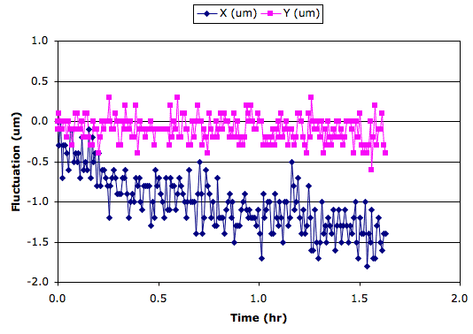
We leave the Acquisifier running our WPS_1.txt every half-hour. We obtain the following plot, which shows the wire drifting downwards and closer to the cameras. After the first hour, the lights in the lab went off for the night. At hour 21, they turned on again when someone entered the lab.

The downward movement may be caused by the aluminum frame cooling and contracting. As the aluminum contracts, the wire sags. The horizontal movement may be caused by the lateral pull upon the wire by its tension screw. As the wire sags, so it moves in response to this lateral pull.
We plucked the wire like a guitar string, as best we could in the vertical direction, waited two seconds, touched the wire, waited five seconds, and measured the wire position. We repeated this procedure many times, and obtained the following graph.
We look down the wire and examine its shape. Instead of a catenary, we see a line that is crooked in both the vertical and horizontal directions. The deviations in the horizontal direction are of order ±200 μm.
We try several times to stretch a wire that is straight and uniform. When we handle the braided carbon-fiber wire, we disturb the braid. The braid and the wire break easily when going around sharp corners. The braid bunches up when we touch it. We cannot smooth out kinks in the wire with our fingers. The only way to get a straight wire is to stretch it as tightly as possible without touching the stretched length at all. We see no bends or kinks in our new wire. The tension in the wire is roughly 100 N. We obtain the following short-term stability plot.
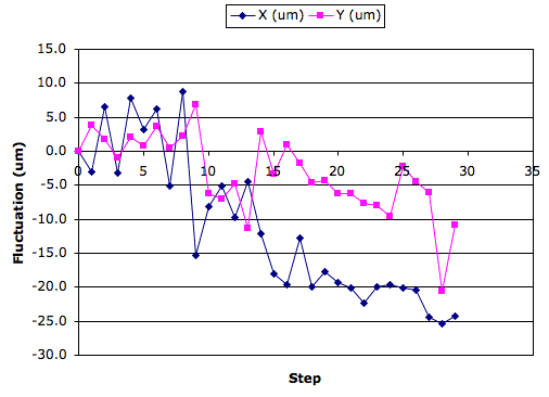
We see the 0.1-μm quantization that results from the WPS script rounding to the nearest 0.1 μm. We increase the resolution of our WPS script's numeric output so that it gives the measurement to 0.01 μm. We see no drift in y, but a 1-μm drift in x over the course of an hour, which is similar to what we saw above. We leave the WPS to run over the weekend.
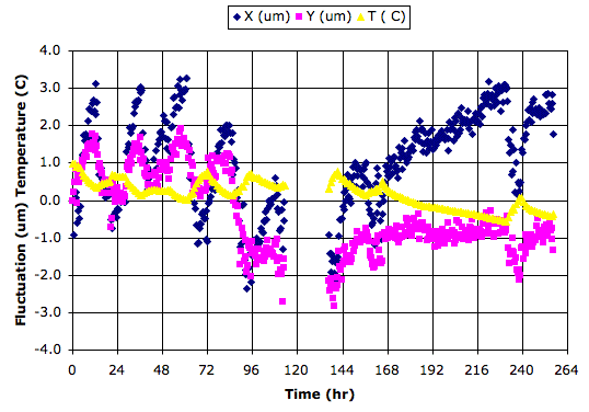
The graph above shows a movements of several microns loosely correlated with temperature at the other end of the laboratory. We do not know if these movements are due to changes in the WPS1 or due to movement of the carbon-fiber wire held in an aluminum frame. We end the experiment after eleven days and move on to an experiment with a steel pin.
We fixed a steel pin in front of the WPS cameras, as shown here. We set the Acquisifier running.
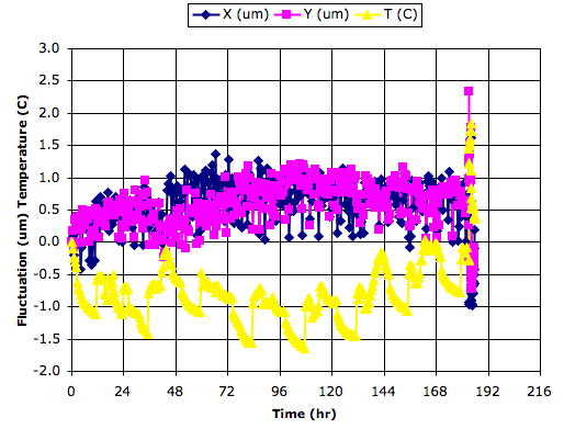
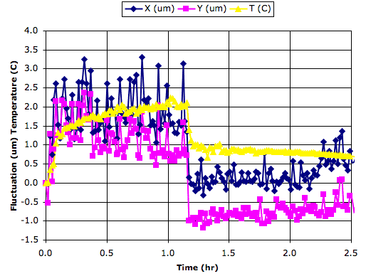
We see 24-hour cycles in temperature, covering a range of 1.5°C. Each working day begins with a sudden rise in temperature of around 0.5°C. Meanwhile, the standard deviation of wire position is only 0.3μm in x and y, with no sign of a 24-hour cycle.
At hour 182 in our experiment, we put a 60 W bulb 30 cm above the WPS1, shining down upon the lid. We increased the frequency of data acquisition to once every 60 s, and left the light on for one hour, and then turned it off. This disturbance is marked by a spike in the temperature and position graphs in the figure above. We present a detail of the disturbance below.
[02-SEP-10] Until now, all the cameras have been glued to the end walls with super-glue. We mark the nominal location of the camera on the end wall with a scribe and ruler, using our drawings. We place the camera on the end-wall and look at a standing wire that we can move along the nominal camera axis. We adjust the camera position and super-glue the camera in place when it is correct. This process was necessary for the WPS1-A because the camera axis was so variable from one camera to the next. We continued with the same process in the WPS1-B. But several cameras broke off during packing and unpacking, and also handling at CERN. Yesterday we repaired P0199, a WPS1-B, by placing the cameras using scribed lines alone and gluing them in place with DP460 24-hour epoxy. We propped the lens holders up with shims. Today we find that the cameras are perfectly positioned and oriented in the WPS xy plane, but pointing slightly in the negative z direction because the shims were too thick. The WPS1-B cameras are uniform in their axis direction because they use a precision and well-centered aperture. Thus we can glue them using scribed lines and a strong, slow-curing epoxy.
[18-OCT-12] For estimates of the effect of temperature upon the measured position of the wire when the sensor is in thermal equilibrium, see Thermal Expansion of the WPS.
[03-MAY-10] As we presented above, the images we obtain with the wire made out of white vectran fibers have poor contrast on account of the wire being almost transparent to the infra-red illumination generated by the WPS1. The focus in these images is sharp enough, but the contrast is so poor that noise masks the sharp edges of the wire image. A longer exposure, in order to obtain more contrast, is not possible because the image sensor begins to saturate with the light reflecting from the WPS1 screen.
We obtained the following series of graphical displays with LWDAQ 7.4.1 operating upon this image. The spot-finding routine used by LWDAQ 7.4.1 allows connection by corner contact between pixels. In do_pixel we set kitty_corner true. This change brings an immediate improvement in the merging of pixel clusters along the edges of dim wire images. But the problem of fragmentation of edge clusters remains for the worst of the images we received from CERN. In order to obtain reliable results with these images, we must merge the edge clusters, which is what the right-hand image shows.
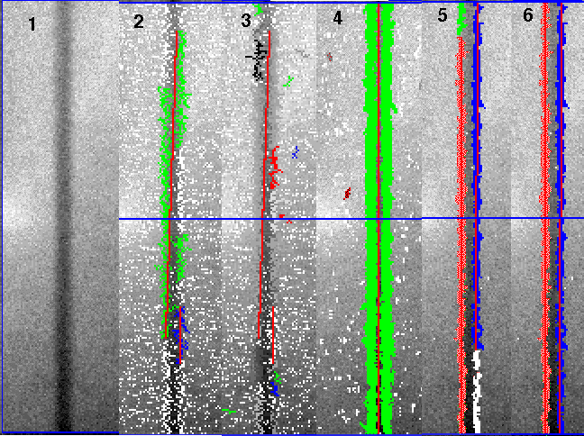
We see the evolution of our low-contrast image analysis from left to right above. With analysis_enable = 2 we introduce smoothing of the derivative image. In result (5) we see that the analysis picks a good selection of edge pixels, but the pixel clusters break into several groups along each wire edge. In LWDAQ 7.4.1 we implemented an algorithm for merging these clusters. With analysis_enable = 3 we activate the merging and we see the result in result (6).
The combination of analysis_threshold "30 # 10" and analysis_enable = 3 becomes the default in LWDAQ 7.4.1. We find that these settings provide robust analysis of all the images we have on disk. The threshold for identifying an edge pixel is 30% of the way from the average to the maximum intensity in the smoothed derivative image. A pixel cluster will be valid only if it contains ten pixels or more. Clusters that coincide with one another will be merged. The bulk of the processing time is spent in taking the derivative of the image and smoothing.
We used the following Toolmaker script to determine the sensitivity of measured edge position to analysis threshold with the improved analysis.
set LWDAQ_config_WPS(analysis_enable) 3
for {set th 1} {$th <= 30} {incr th} {
	set LWDAQ_config_WPS(analysis_threshold) "$th \$ 10"
	set result [LWDAQ_acquire WPS]
	LWDAQ_print $t "$th [lindex $result 1] [lindex $result 7]"
}
The test code uses the "$" threshold specifier, which sets the threshold equal to a number of counts above the average intensity in the image. We obtained the following graph by applying the code to this image of a white vectran wire taken with a WPS1-B at CERN.
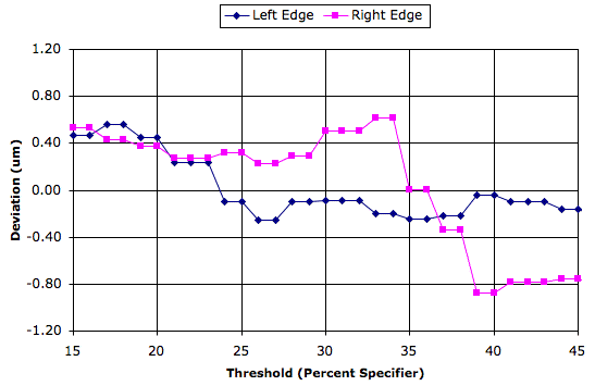
Outside the range plotted above, the analysis begins to fail and we obtain large errors in position. Within this range of 15% to 45%, the standard deviation of the position is under 0.5 μm, which corresponds to a standard deviation in wire center position of around 5 × 0.5 μm / √2 = 1.8 μm.
We used the following Toolmaker script to see how exposure time affected the measured position of a wire edge.
set LWDAQ_config_WPS(analysis_enable) 3
set LWDAQ_config_WPS(analysis_threshold) "30 \# 10"
for {set fs 0.01} {$fs <= 1} {set fs [expr $fs * 1.1]} {
	set LWDAQ_config_WPS(daq_flash_seconds) $fs
	set result [LWDAQ_acquire WPS]
	LWDAQ_print $t "[format %.2f $fs] [lindex $result 1] [lindex $result 7]"
}
We obtained the following graph for two different wires as we varied the exposure time from 10 ms to 1 s using a WPS1-B.
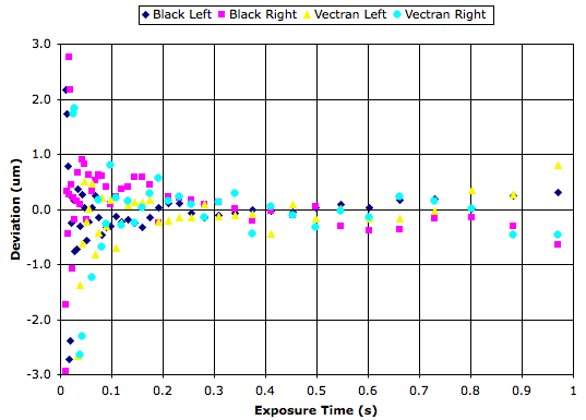
The WPS1-B begins to saturate at around 900 ms. We can see vertical white stripes in the image. The plot suggests and optimal exposure time of around 400 ms. The WPS1-C has a larger aperture. It saturates at around 400 ms, which suggests an optimal exposure time of around 200 ms.
We used the following code to compare the performance of the analysis with and without merging. We acquired images from a WPS1-B looking at a white vectran wire with exposure time 100 ms.
button $f.stop -text Stop -command "set count 100"
pack $f.stop
for {set count 1} {$count <= 100} {incr count} {
	LWDAQ_print -nonewline $t "$count "
	set LWDAQ_config_WPS(analysis_enable) 2
	set LWDAQ_config_WPS(analysis_threshold) "30 \# 10"
	set result [LWDAQ_acquire WPS]
	LWDAQ_print -nonewline $t "[lindex $result 1] [lindex $result 7] "
	set LWDAQ_config_WPS(analysis_enable) 3
	set result [LWDAQ_analysis_WPS]
	LWDAQ_print $t "[lindex $result 0] [lindex $result 6] "
}
The experiment took roughly one minute to run. The left edge of the wire suffered very few fragmentations of its pixel clusters, but fragmentation was frequent on the right edge. The following table summarizes our observations.
| Property | Left Edge No Merging |
Left Edge With Merging |
Right Edge No Merging |
Right Edge With Merging |
|---|---|---|---|---|
| Average (μm) | 1935.46 | 1935.05 | 2048.76 | 2052.40 |
| Standar Deviation (μm) | 0.6 | 0.4 | 4.0 | 0.9 |
| Spread (μm) | 3.2 | 2.4 | 13.0 | 4.5 |
The merging improves the resolution of the right edge by a factor of three or four, and provides a slight improvement in the left edge. What is more striking is the change in the average value of the right edge position. The edge appears to move 4 μm to the right when we include all available edge pixels. We increase the exposure time to 400 ms, which we think is ideal for the WPS1-B, and obtain the following results.
| Property | Left Edge No Merging |
Left Edge With Merging |
Right Edge No Merging |
Right Edge With Merging |
|---|---|---|---|---|
| Average (μm) | 1935.02 | 1935.00 | 2052.31 | 2052.31 |
| Standar Deviation (μm) | 0.18 | 0.13 | 0.20 | 0.20 |
| Spread (μm) | 1.6 | 0.7 | 1.0 | 1.0 |
With four times more contrast, merging corrects rare errors in edge measurement.
Here we discuss and present the results of tests of the WPS1 at other laboratories. Here is a list of available documents from those laboratories.
[25-MAY-10] One thing they observe at CERN repeatedly when working with all manner of wires are bands in the deviation of measured wire position from its average value, as you can see on page 2 here. These bands are separated by several microns. We cannot reproduce these bands in our laboratory, even with white Vectran wire and exposure time less than half the recommended duration. Even when the exposure time is so short that we see failure of image analysis, the deviation in wire position appears gaussian in its distribution and we see no sign of bands. We suspect a problem in software, when the two wire planes obtained from the two cameras are intersected by the CERN data-analysis code.
We prepare an Acquisifier script, WPS_4.txt, that performs this intersection for itself. The result string of one run through the script has the form "timestamp name1 x1 y1 name2 x2 y2", where name1 is the name of the first WPS, x1 is the x-position of the wire in mount coordinates where it intersects the z = −5 mm reference plane, and y1 is the y-position of the wire.
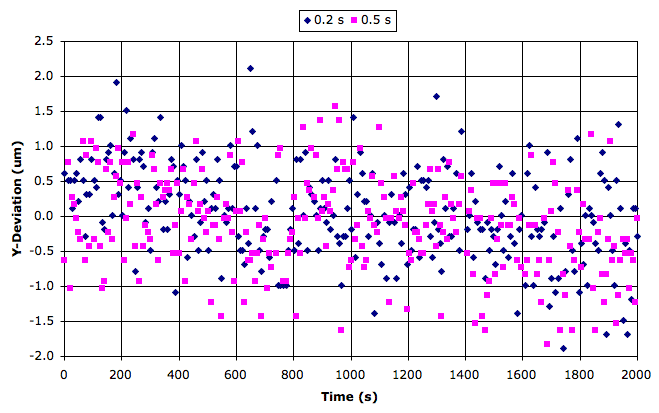
We obtained the above graph with a modified version of WPS_4.txt. The script first measures the position of the wire with 200 ms exposure, then with 500 ms exposure. We see no sign of bands in the deviation, other than the 0.1-μm bands due to our rounding the wire position to the nearest 0.1 μm.
[28-MAY-10] With WPS_4.txt, CERN sees no sign of the deviation bands, as they report here.
[22-JUN-10] CERN gets better long-term results with the new script, as they show in the New DAQ section here. Sensor measurements now cover a spread of 2 μ to 6 μm when monitoring the vectran wire. The WPS1-A does better than the WPS1-B, on account of its larger aperture. In their tests over several days, the wire they were monitoring moved down a few microns. For WPS1-B graph of deviations see here, for WPS1-A see here.
[09-JAN-08] We delivered our prototype WPS1 to Helene Durand at CERN. Her colleague Friedrich Lackner mounted the WPS1 upside-down on a CMM along with a wire, as shown in his photograph.
[01-MAR-08] We have three more WPS1s assembled and tested.
[26-MAR-08] We receive an order for two calibrated WPS1 from CERN.
[10-APR-08] Begin stability tests with steel dowel pins.
[01-MAY-08] Satisfied that resolution and stability of WPS1 is better than 1 μm rms for ±1°C.
[20-MAY-08] Obtain first calibration data from CMM with dowel pins and WPS1 on translation stage. Begin dedicated Calibration page.
[26-JUN-08] Investigating non-linearity in camera optics, which we believe to be the result of lens aberration.
[03-DEC-08] CERN approves order of 8 more WPS1. OSI designs lens holder with precision pinhole aperture. Accurate centering of the aperture should reduce wedge-angle aberration to less than 3 μm in wire position.
[09-APR-09] Have completed construction of 8 WPS1 for CERN. Of these, 7 are WPS1-B and 1 is WPS1-A. The WPS1-Bs are calibrated to 2 μm accuracy across the entire field of view. The WPS1-A is calibrate to 4.5 μm.
[12-AUG-09] Prepare WPS_3.txt data acquisition script for multiple-WPS test stand at CERN, where Patric Bestmann and Andreas Herty have three WPS1-Bs under test, as shown here.
[12-NOV-09] CERN has been working with three WPS1s to study their performance.
[03-FEB-10] DESY orders 2 WPS1-B. We will deliver 2 WPS1-C devices, with larger apertures, more able to view white vectran wire.
[12-MAR-10] Patrick Bestmann, Andreas Herty, and Freidrich Lackner produce a report on the resolution and dynamic range of the WPS1-B. They appear to be having trouble analyzing images they obtain from their white vectran fiber, which is transparent to infra-red light.
[16-APR-10] We have images from CERN that show poor enough contrast that the edge pixel clusters along one or other edge of the wire image tend to separate into two or more separate clusters. We will implement logic to re-combine these clusters and recover the entire edge for better performance.
[03-MAY-10] Test new cluster-merging routine on the CERN images and find that it is always able to combine the edge pixels along each side of the wire image. Report on this in Low-Contrast Images.
[11-MAY-10] Calibrate first WPS1-C. Obtain 1.0 μm ray error for each camera, 1.6 μm line error for both cameras combined, over 22 pin positions.
[14-MAY-10] Ship 2 WPS1-C to DESY.
[20-MAY-10] Receive a report from CERN on performance of new edge-merging analysis. They still see discrete bands in the deviation of wire position from average.
[25-MAY-10] New readout script includes calculation of wire position for arbitrary number of WPS devices, WPS_4.txt.
[27-JUL-10] CERN has lent two WPS-Bs to SLAC. We hear from Georg Gassner, "So far we only did some static tests, the sensors seem to perform quite well. We have the vectran wire from CERN but I think it is white."
[08-JAN-11] We received two WPS1-Cs back from DESY. Each had suffered a broken-off camera. We broke off all the cameras and glued them with DP460 Epoxy. Today we re-calibrated the two sensors and will ship them back.
Our WPS1 resolution is better than 1 μm in measuring the vertical and horizontal position of a wire. Friedrich Lackner at CERN obtained better than 1-μm stability over three weeks, as he reports on his new WPS wiki. We obtained better than 1-μm accuracy while monitoring the position of a dowel pin mounted to the WPS1 base. Systematic errors due to stray illumination of the wire, shadows on the screen, non-uniform illumination of the screen, changes in image brightness, and choice of analysis threshold combine to give an error less than 5 μm in wire position, or 1 μm on the image sensor. Our derivative analysis of WPS1 images finds the left and right edges of a wire or pin. The analysis produces accurate, robust results, and runs in roughly 10 ms on a 1.3 GHz G4 lap-top.
The WPS1 dynamic range is roughly 20 mm wide and 14 mm high. The dynamic range is not square or circular, but rather a pentagon defined by the intersection of the two camera fields of view and the passage of the cover as we lower it onto the base. As a result of variation in our assembly process, the location of this dynamic range varies from one device to another by ±2 mm WPS1-A. There is at least a ±5 mm range that will be enclosed in the dynamic range of all WPS1s.
We calibrated four WPS1-As and eight WPS1-Bs with the help of black steel pins and our CMM, as we describe in WPS1 Calibration. By modeling each WPS1 camera with nine parameters, and using twenty-two wire positions to calculate these parameters, we obtain 2 μm absolute accuracy across a 7 mm × 12 mm area with our WPS1-B optics and better than 10 μm accuracy with our WPS1-A optics.
Readout from a system of multiple WPS1s can be carried out with the LWDAQ software's Acquisifier. In our demonstration script, the Acquisifier uses camera calibration constants to calculate a plane containing the wire center-line for each image it obtains. Another program, perhaps running within LWDAQ or perhaps making use of the result file created by the Acquisifier, calculates the intersections of these planes to obtain wire positions.
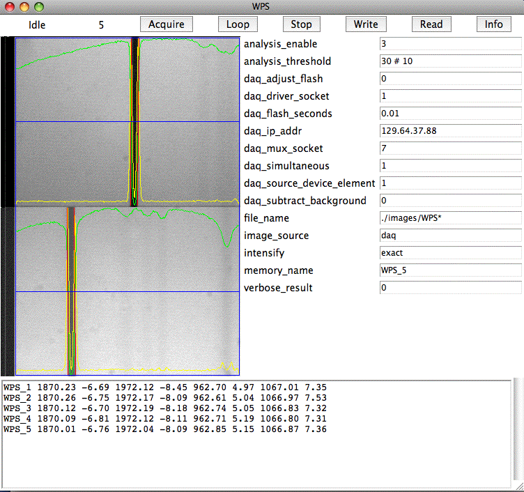