Implantable Lamp (A3024)
© 2012-2017 Kevan Hashemi,
Open Source Instruments Inc.
Contents
Description
Design
Frequency Tuning
Antenna Matching
Lamp Current
Switching Noise
Optical Power
Head Fixture
Battery Life
Encapsulation
Fiber Construction
Conclusion
Appendix: Batch ISL4C
Appendix: Batch ISL5
Appendix: Batch ISL6
Appendix: Batch ISL7
Description
The Implantable Lamp (A3024) is a radio-controlled lamp powered by a battery. Once encapsulated in epoxy and silicone, it is water-proof and compact, so so that it may be implanted in an animal. The A3024 can, in theory, be activated by any sufficiently-powerful source of radio waves. But we plan to activate the A3024 with the Command Transmitter (A3023CT), which produces 146-MHz radio waves. Thus the tuning circuit shown in the S3024 circuit diagram is designed to select power in the neighborhood of 146 MHz.

Figure: Implantable Lamp Circuit, A3024A. Divisions are millimeters. The leads are helical steel insulated in silicone, 150 mm long, resistance 30 Ω and terminated with pins for connection to a Head Fixture (A3024HF). The encapsulation is black epoxy and four coats of silicone. The battery is a BR1225 with capacity 48 mA-hr. The antenna is 200 mm of stranded stainless steel wire wound in two loops of diameter 30 mm.
The A3024 is useful in its own right as an implantable source of optical stimulation for gene therapy. It is intended, however, to test the command reception, lamp power generation, and light delivery of the Implantable Sensor with Lamp (ISL). Delivery of the A3024 is part of the ISL development, as detailed in the ISL Technical Proposal

Figure: Head Fixture (A3024HF). Two sockets mate with the Implantable Lamp Circuit (A3024A) pins. This is the original version, with the guide cannula separated from the fiber tip.
The A3024 provides 5-V power to an LED through its L+ and L− pads. These must be connected to two leads with resistance suitable for driving the lamp with 5 V. If the forward voltage drop of the LED is 3.1 V and we want 20 mA current, the lead resistance should be around 100 Ω.
In the ISL Conceptual Design, we proposed to use the L+ lead as an antenna for command reception. But this turns out to be impractical. The input impedance of our tuning circuit is around 10 kΩ. In order to force 146-MHz power to pass through the tuning circuit rather than into the lamp power supply, we would need a 10-μH inductor with self-resonant frequency 150 MHz or higher on both the L+ and the L− inputs. We can't find such an inductor in a surface mount package. The A3024 provides two pads for a small loop antenna. One is connected to the tuning circuit, the other to the circuit ground.
Function
Code |
Tuning (MHz) |
Battery
Capacity
(mA-hr) |
Volume
(ml) |
Lamp
Life (hr) |
Shelf
Life (mo) |
| A3024X |
None |
1000 |
− |
72 (30 mA @ 10%) |
560 |
| A3024Y |
None |
48 |
1.7 |
1.7 (30 mA @ 10%) |
27 |
| A3024A |
Gain >4 @ 146 MHz |
48 |
1.7 |
1.7 (30 mA @ 10%) |
27 |
| A3024B-M |
Gain >4 @ 146 MHz |
19 |
1.7 |
2.2 (42 mA @ 10%) |
27 |
| A3024B-R |
Gain >4 @ 146 MHz |
160 |
4.8 |
20 (42 mA @ 10%) |
27 |
Table: Versions of the A3024 Implantable Lamp.
The table above lists the defined versions of the A3024. The shelf life is the time it will take the quiescent current of the device to run down the battery if the lamp is ever turned on. We estimate shelf life by dividing the battery capacity by the measured A3024 inactive battery current of 2.5 μA. The lamp life is the time it will take to run down the battery with the lamp flashing for 1 ms every 10 ms. Because different lamp and wire arrangements result in a different lamp current, we specify a lamp current at which we measured the average battery current. We divide the battery capacity by this active current, and then divide by two again (see below). We do not specify volume for versions that are not encapsulated.
Design
S3024A_1: Circuit diagram for A3024A, with tank tuning circuit, lithium primary cell, and 1-mF capacitor bank.
S3024B_1: Circuit diagram for A3024B, with split capacitor tuning circuit, lithium-ion secondary cell, no capacitor bank.
S302401A: Gerber files for PCB version A.
S302401A_GTO: Top silk screen of PCB version A.
S302401A_GBO: Bottom Silk Screen of PCB version A.
S302401A.BOM: Bill of materials for PCB version A.
S302402A.zip: Head Fixure PCB Version A.
S302402B.zip: Head Fixure PCB Version B.
S302402C.zip: Head Fixure PCB Version C.
S302402C.png: Head Fixure Version C Drawing.
LTC3525-5: Inductive boost regulator that supplies power to lamp.
MCP6541: Micropower comparator.
HSMS285C: Zero-bias detector diode.
EZ290: High-efficiency chip LEDs for coupling to optical fiber, green and blue.
EZ500: High-efficiency chip LEDs for coupling to optical fiber, green and blue.
Conceptual Design: The thinking behind this circuit, including crystal radio, capacitor bank, and boost regulator.
Frequency Tuning
The A3024 tuner consists of R4, L2, and C14. The detector is D2 with C13, as shown in the S3024A circuit diagram. The photograph below shows the tuner assembled on the circuit board, using two 5 pF capacitors and one 2 pF capacitor to make 12 pF. The 100 nH inductor is beneath one of the capacitors.
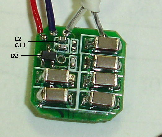
Figure: Tuner Side of the A3024. This is the side that will be covered by the battery. The large components are the 100-μF capacitors of the capacitor bank. The circuit is 12 mm wide.
[04-JAN-13] We solder a two-loop 3-cm diameter detection antenna to the A and GND terminals of our A3024 circuit board. We load R4, C13 and D2 into the circuit, but not the tuning capacitor C14 and tuning inductor L2. We still have a DC path to ground for the diode through the antenna, so that the diode resistance and R4 form a low-pass filter with C13.
We set up our Command Transmitter (A3023CT) with a 3-dB attenuator and rubber ducky antenna attached to its +22-dB output. We do not use the A3023CT's booster amplifier. We load the comparator that detects the presense of radio-frequency power and the boost regulator that powers the lamp. We attach a battery, as shown below. The lamp turns on with RF power.
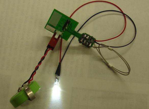
Figure: Implantable Lamp, A3024X. The lamp consists of two 30-Ω leads and a while LED. The external battery is a BR2477. Note the capacitor soldered between the LED leads.
[04-JAN-13] We take an A3019E transmitter and place its antenna adjacent to our 2-loop A3024X antenna. We are looking to see if we can turn on the lamp with its 915-MHz transmission, given that we have no tuning ciruit on the A3024X. We see a signal correspondig to the A3019E transmission of amplitude roughly 2 mV on VR. This 2 mV is unsufficient to turn the lamp on.
[16-JAN-13] We remove the battery from our A3024X so that the comparator and boost regulator are without power. We connect the output of our Command Transmitter A3023CT through a 14-dB attenuator to an 80-mm length of wire that we loop around our A3024X antenna so as to transfer RF power between the two antennas and not between the A3023CT and our oscilloscope probes. We sweep the A3023CT output frequency from 120 MHz to 200 MHz and record VR.
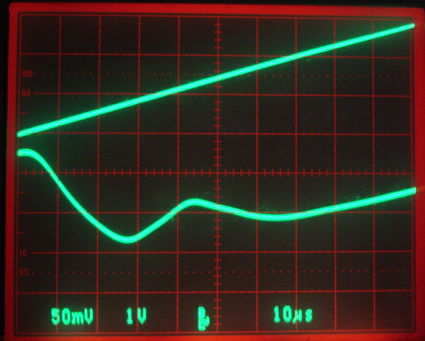
Figure: Detector Output (VR) and VCO Control (TUNE) with No Tuning Capacitor or Inductor. Top trace is TUNE, 0 V to 3 V sweep gives roughly 120 MHz to 200 MHz. The frequency is 146 MHz when TUNE is 1.25 V. Bottom trace is VR, 50 mV/div, with the voltage in the center of the field being 120 mV.
The frequency response above would ideally be flat, but we have the frequency-dependence of the VCO output amplitude, the amplifier gain, and the antenna impedances. These appear to combine to give us variation in received RF power.
[16-JAN-13] We load C14 = 5 pF and L2 = 100 nF and repeat the above experiment. We are expecting the peak response to be at 146 MHz because these are the values that gave us a peak response at 146 MHz in our Command Receiver (A3023CR). But instead the peak is out of our sweep range.
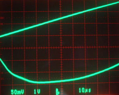
Figure: Detector Output (VR) and VCO Control (TUNE) for 5-pF tuning capacitor and 100-nF tuning inductor. Top trace is TUNE, 0 V to 3 V sweep gives roughly 120 MHz to 200 MHz. The frequency is 146 MHz when TUNE is 1.25 V. Bottom trace is VR, 50 mV/div, with the voltage in the center of the field being 10 mV.
According to our calculations, the correct capacitance for resonance at 146 MHz with a 100-nH inductor is 12 pF. So we add another 5 pF and 2 pF to make a total of 12 pF. We obtain the following tuning curve.
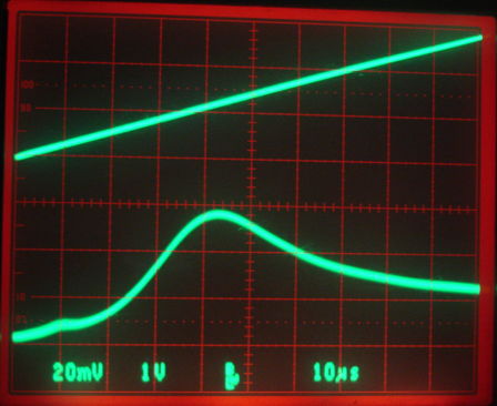
Figure: Detector Output (VR) and VCO Control (TUNE) for 12-pF tuning capacitor and 100-nF tuning inductor. Top trace is TUNE, 0 V to 3 V sweep gives roughly 120 MHz to 200 MHz. The frequency is 146 MHz when TUNE is 1.25 V. Bottom trace is VR, 20 mV/div, with the voltage at the peak being 65 mV (0 mV is not on one of the scale lines).
Now we see a peak response at almost exactly 146 MHz, and using component values that agree with our calculations. But we note that the peak voltage is only 65 mV, and this is after we fiddle with the antennas to get the biggest signal. We obtained 120 mV at 146 MHz with not fiddling when we had no tuner.
We try again to activate the lamp with the antenna of an A3019E. We see no sign of the A3019E transmission in VR. Whatever signal the A3019E induces is less than 2 mV. The lamp will not turn on.
We measure reception range for the same antenna orientations and power. We see the lamp flashing at range 12 cm with our tuning circuit in place, 13 cm with the tuning circuit removed, and 17 cm when we cut off the extension circuit, load a BR1225 battery, and leave off the tuning circuit.
[17-JAN-13] After clipping off the extension and loading a battery onto our A3024, we have an A3024Y. It has no tuning circuit. We use our 1/2-wave antenna and booster amplifier to provide as much 146 MHz power as we can. We attach the circuit to the end of a stick and pulse the RF power for 5 ms out of every 50 ms. After about ten minutes of moving around, we estimate that reception is at least 95% reliable at ranges 50 cm and less. We load the tuning circuit and repeat our movements. Reception is now only 80% at 50 cm. We remove the tuning circuits. Reception jumps back up to over 95%.
[18-JAN-13] We turn on our A3023CT and add 30 dB of attenuition. We sweep the A3023CT frequency with our function generator. We obtain the following trace of TUNE and RF. The center of the trace corresponds to 146 MHz and our RF power is −8.5 dBm.
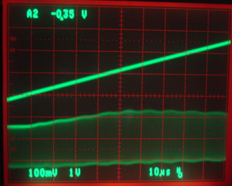
Figure: TUNE and RF. Top trace TUNE, 1 V/div. Bottom trace is RF, 100 mV/div. At center, TUNE is 1.25 V, RF is 146 MHz and −8.5 dBm.
We start a new A3024X assembly. We load D2, R4, and C13. We connect our RF power to the antenna input with an adjacent 50-Ω terminator to provide a ground path for VR.
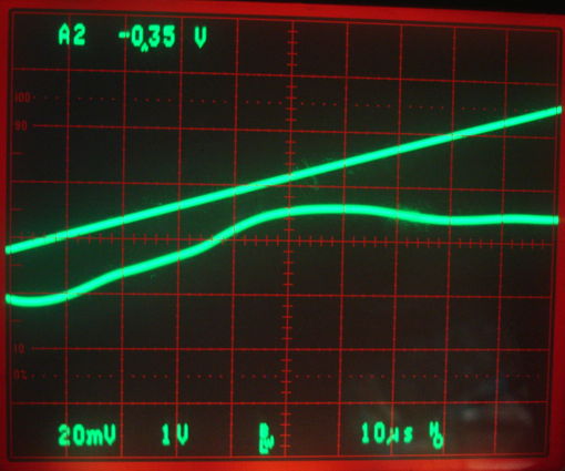
Figure: TUNE and VR with No Tuning. Top trace TUNE, 1 V/div. Bottom trace is VR, 20 mV/div. At center, VR is 71 mV.
Consulting the graph of VR versus RF amplitude we present here, we see that our 120-mV amplitude RF signal should produce detector voltage close to 73 mV, and this is what we observe. Now we load 12 pF and 100 nH into C14 and L2. We now obtain the following trace for VR.
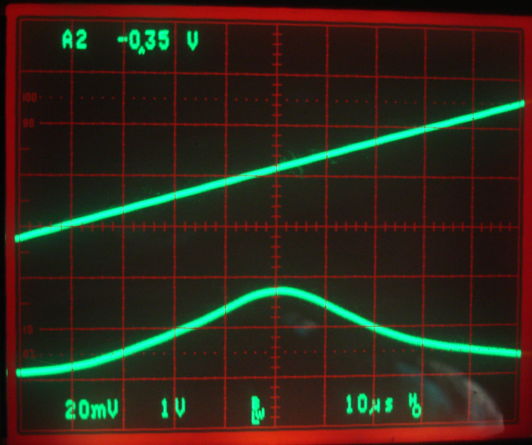
Figure: TUNE and VR with P0402 Inductor Tuning. Top trace TUNE, 1 V/div. Bottom trace is VR, 20 mV/div. At center, VR is 34 mV.
We see resonance at 146 MHz. But we now have VR only 34 mV, which suggests that the RF input to the detector diode has amplitude only 70 mV. With 140 mV at the antenna and 70 mV on the tank circuit, the impedance of the tank circuit at resonance is the same as R4, or 1 kΩ. The tank circuit of the A3023CR gave us an impedance of order 10 kΩ at resonance. On the A3024 we are using the ELJ-RFR10GFB (P0402 package). Its self-resonant frequency is 1200 MHz. The A3023 uses the AISC-0805-R10J-T (P0805 package). Its self-resonant frequency is also 1200 MHz, but its minimum Q at 250 MHz is 50. With some fiddling about, we load the larger inductor onto our A3024 and try various capacitors. With C14 = 11 pF we obtain the following traces.
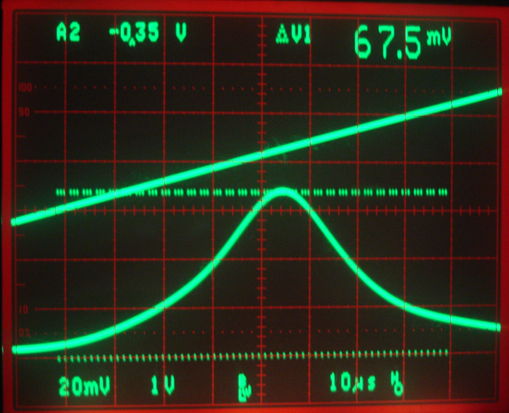
Figure: TUNE and VR with P0805 Inductor Tuning. Top trace TUNE, 1 V/div. Bottom trace is VR, 20 mV/div. At center, VR is 68 mV.
With VR at 68 mV, the RF amplitude on the tank circuit should be around 110 mV. Given that we are applying 120 mV amplitude to R4, we conclude that the impedance of the diode and tank circuit in parallel at resonance must around 11 kΩ. Given that this is greater than the typical 8-kΩ video resistance of our detector diode, we see that the impedance of the tank circuit at resonance must be much greater than 11 kΩ.
By losing 50% of the amplitude of our incoming RF signal, the P0402 tuner loses 75% of the power received by our antenna. We expect the tuner to reduce the effective range of the implantable lamp by a factor of two.
[24-JAN-13] We set up our Command Transmitter (A3023CT) with a frequency sweep and 30-dB attenuator. We obtain a 67-mV peak at 146 MHz with our P0805, 100-nH inductor and 11 pF capacitor. We try out some new P0402 inductors. With the LQW15ANR10J00D and 12 pF we obtain a peak of 50 mV. With the CW100505-R10J we get 52 mV. With the 744765210A we get 48 mV. We fix a broken wire in our RF delivery. With the P0805 inductor we now get only 64 mV at around 147 MHz. We try another P0805 inductor with 12 pF instead of 11 pF and we get 61 mV at 144 MHz. We conclude that we need a P0805 inductor for efficient tuning. We can load one onto the A3024 circuit because of a fortunate feature of the layout.
[24-JAN-13] As we report here, today we set up our first faraday canopy enclosure and tried out the A3024Y inside. Reception is about the same as outside. The A3024Y is encapsulated and has no tuning, so it is in theory receptive of any RF power it picks up. We place it on top of our Airport Express wireless base station, and the lamp flashes with 2.4 GHz power generated by WiFi activity. Inside the enclosure, it never flashed except when we stimulate it with our ownn 146 MHz.
Within the enclosure, we hold the A3024Y between thumb and forefinger and move it at random 30 cm from the transmitting antenna. We obtain 100% reliable reception. We move to range 50 cm and obtain 95% reliable reception. If we hold the A3024Y in our hand, enclosing its two-loop receiving antenna, reception at 30 cm drops to 95% and at 50 cm drops to around 80%. We expect that reception from an implanted A3034Y would be somewhere in between these two tests.
Antenna Matching
[28-JAN-13] The resistor with tank tuner operates by attenuating the antenna signal at frequencies other than 146 MHz. The resistor and the tank act like a voltage divider. At 146 MHz, the tank resonates and its impedance is greater than the 10 kΩ resistance of the tuning diode. The voltage on the tank circuit is roughly 90% of the voltage on the antenna. At other frequencies, the impedance of the tank is much smaller than 1 kΩ. The voltage on the tank circuit is much smaller than the antenna voltage.
We now look at ways we can use inductors and capacitors to amplify the antenna voltage so as to increase our operating range. Such amplification is possible with passive components provided that the source resistance of the antenna signal is less than the load resistance of our tuning diode. Our two-turn loop antenna is 33 mm in diameter, made out of 200 mm of 360-μm diameter stranded stainless steel wire. At 146 MHz, the skin effect drives electrical current to the surface of the conductors, increasing the effective resistance of the wire. The resistance per unit length of solid wire becomes:
R = √(ρ f μ) / (4 r √π)
where ρ is resistivity, f is frequency, r is the wire radius, and μ is the permeability of the metal. The resistivity of 316SS is 740 nΩm (compare to 17 nΩm for copper). Its permeability for stattic magnetic fields is 200. We can pick it up with a strong magnet. But at radio frequencies, its permeability is close to 1. Our antenna is stranded, but it turns out that this does not make much difference to the skin effect. Our wire is 200 mm long, so its resistance at 146 MHz should be around 100 Ω.
As we discuss in elsewhere, the antenna signal itself has a source resistance, which we call the radiation resistance. But for our small loop antenna at 146 MHz, the radiation resistance will be less than 1 Ω, which is much smaller than the resistance of the steel wire.
The self-inductance of a wire loop is easy to think about but hard to derive with analytic equations. There are good approximations available, however, and we can use calculators like this one to obtain an estimate of loop inductance. Such calculations suggest that our two-turn antenna has inductance 300 nH.
In an earlier discussion of the ISL antenna, we considered the capacitance between an open-ended antenna and the nearest ground potential. In the case of our loop antenna, this capacitance is in parallel with a direct connection to the tuner's ground potential by the antenna wire. The capacitance will be the capacitance between the antenna coils and the tuner circuit, and so will be or order 1 pF. Its reactance will be of order −1 kΩ and will act in parallel with roughly half the loss resistance of the antenna, which is 50 Ω.
We neglect antenna capacitance and radiation resistance in our loop antenna, and model it with three lumped components: a voltage source, a self-inductance of 300 nH, and a loss resistance of 100 Ω. Given that our diode resistance is 10 kΩ, we see that we can hope to build some circuit out of inductors and capacitors that will amplify the antenna voltage for our detector diode. This circuit will transform the current and voltage it draws from the antenna into a signal of the same frequency with higher voltage and proportionally lower current.
[28-JAN-13] We analyze the following matching circuit. The signal VA represents the voltage induced upon our antenna by radio waves. Component L1 represents the self-inductance of our antenna. Component R2 represent its loss resistance. We have a series resistance we can insert deliberately in R3. The two capacitors C1 and C2 form a divider and also resonate with L2. Resistor R1 is our detector diode. The voltage VT is the signal on the input of the diode.
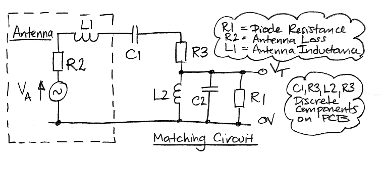
Figure: Antenna Matching Circuit. Note that component names do not correspond to those we use in the S3024A_1 schematic.
We obtain the following expression for the complex gain of the circuit. We have done little to tidy it up, but we have tested it in a dozen different ways, so we are confident it is correct, despite its complexit. You will find this equation implemented in this spreadsheet.
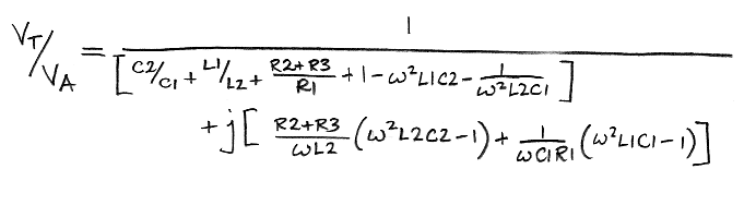
Figure: Antenna Matching Gain. Here j is the square root of −1 and represents a +90° phase shift between voltage and current.
The following plots show how the gain from VA to VT for various combinations of components, including our original resistor with tank circuit. The most striking prediction of the analysis is that we will see sharp, resonant amplification when we make C1 small, and that this resonance is only weakly dependent upon the nature of the antenna.
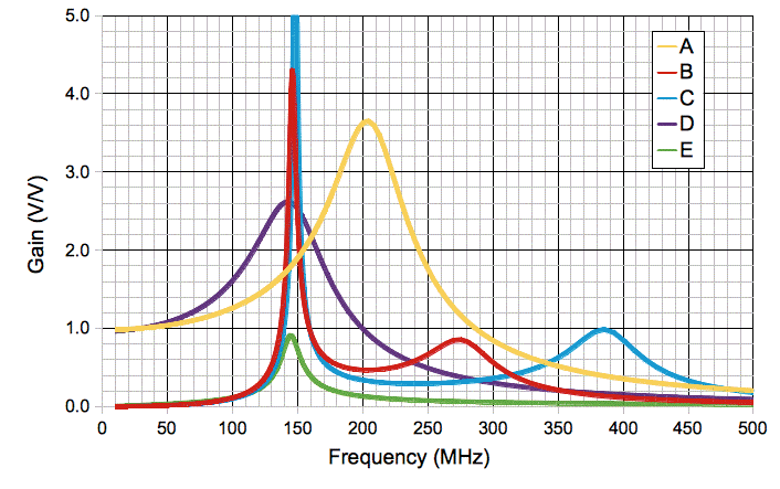
Figure: Antenna Matching Gain, For Various Configurations, 0-1000 MHz. We plot the absolute value of the gain. Component values we use to obtain the plots given in table below. Plots D and E lie on top of one another in the neighborhood of 150 MHz.
The table below gives the component values that we used to obtain each plot.
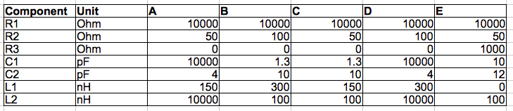
Table: Component Values Used in Plots Above and Below. Component names given in the antenna matching circuit diagram.
Trace E shows our resistor and tank tuner connected to a coaxial cable signal source. We set the antenna inductance to zero and its resistance to 50 Ω to represent the source impedance. We set the series capacitor and resistor as we did in our original tuning experiments, and we obtain a graph that looks very much like the one we observed.
Trace D shows resonance of the antenna with C2 alone. We have made L2 so large that its impedance is effectively infinite, and omitted C1 and R3. The 300-nH inductance of the antenna and the 4-pF capacitance of C2 resonate at around 140 MHz and give us gain of more than 1.0 at 146 MHz. The peak would be sharper and higher, but our antenna resistance of 100 Ω damps the resonance so that the peak gain is only 2.6. Trace A shows us how sensitive such antenna resonance is to the properties of the antenna itself. Here we switch from a two-loop antenna to a single-loop antenna, so that the antenna resistance is 50 Ω and inductance is 150 nH. The resonant peak moves to 200 MHz and 3.7. But we note that we still have gain greater than 1.0 with this resonance at 146 MHz.
Trace B illustrates antenna matching by a small capacitor in series with a larger capacitor. We call this the "split capacitor" network, and it operates with its own resonant inductor. We set C1 to 1.3 pF and C2 to 10 pF. These two in parallel resonate with our 100 nH L2 at 146 MHz. But C1 and C2 also act as a capacitive divider. The gain at resonance is around 4.2 with phase −111° with respect to the antenna signal. The voltage across C1 is 4.6 times larger than the antenna voltage with a phase of −57°. The current flowing through it has phase +32°. Thus C1 presents to the antenna an impedance to ground that is much smaller than that of C1 alone, and has a real component that is much smaller than that of R1. Thus C1 acts to match the impedance of the antenna to that of our diode. There is a second resonance in this matching network, when the antenna impedance resonates with C1. This resonance is at a higher frequency because C1 is so small.
Trace C shows how insensitive the two-capacitor matching circuit is to the antenna properties. We try a single-loop antenna and the resonant frequency moves up only by a few megahertz. The peak gets higher in our calculation because the antenna loss resistance is less. We see the secondary resonance of the antenna inductance jumping up in frequency because the antenna inductance has halved.
[28-JAN-13] We load 1 pF into the R4 footprint of an A302401A printed circuit board, and 8 pF into C14. We have 100 nH in a P0805 package for L2. We connect our two-turn, loop antenna and orient it straight up. We use our Command Transmitter (A3023CT) to produce 22 dBm of RF power, which we feed through a 12-dB attenuator into a rubber ducky antenna. The receive antenna faces the transmit antenna at a range of 33 cm. We obtain the following response.

Figure: Response of Split-Capacitor Matching Network. Referring to the circuit diagram above (rather than the A3024 schematic), we have C1 = 1 pF, C2 = 8 pF, L2 = 100 nH and R3 = 0 Ω. The antenna inductance and resistance are provided by the actual antenna. Top trace is the VCO tuning voltage, sweeping from 0-4 V in 1 ms. Frequency varies from 116-198 MHz, with 146 MHz at 1.25 V.
We see two peaks in the response, one of 300 mV close to 146 MHz, and one of 120 mV close to 170 MHz. When we remove the split capacitor and replace it with our resistor-tank tuner, we get a peak at 40 mV. Using the detector diode response plot, we see that a 300-mV peak on VR implies VT amplitude 400 mV, 120-mV implies amplitude 200 mV, and a 40-mV peak implies amplitude 80 mV. Given that our tank tuner has peak gain 0.9, we see that our split capacitor tuning circuit appears to be giving us gain 4.5 at 146 MHz and 2.5 at 170 MHz.
When we insert the above component values into our spreadsheet calculator, and assume antenna inductance 300 nH and resistance 100 Ω, we get peaks of 4.6 at 162 MHz and 0.9 at 310 MHz. Thus our calculation does not agree exactly with observed response, but it is pretty close.
We load the rest of the components onto the circuit to create a completed A3024 with the split-capacitor tuning. We set the Command Transmitter (A3023CT) to transmit 1 ms pulses of 146 MHz power every 10 ms. We connect an external battery to the A3024. We solder a blue LED with a 200 Ω resistor to the L output. We connect our two-loop antenna.
We wander around the laboratory. Twenty meters away, far back behind the dividing cabinets, we get 10% reception. At 14 m 50%, at 6 m 95% and at 3 m or closer 100%. We put the receiver in our small faraday enclosure, and reception is 0%. We conclude that the split capacitor matching network is effective, and increases our operating range by at least a factor of five.
[30-JAN-13] We set up our faraday canopy and try the tuned A3024 within the canopy with 32 dBm on our 1/2-wave antenna. Reception is 100% reliable within the enclosure. We try again with 10 dBm on our antenna and reception is 100% reliable within the enclosure except when we bring the A3024 loop antenna within a few centimeters of the absorber on the floor, with the coil oriented in a vertical plane facing the transmitting antenna.
[31-JAN-13] We equip our tuned A3024 with a new antenna soldered to its antenna pads. We find that we must increase C14 from 8 pF ot 9 pF to put our peak gain at 146 MHz. We encapsulate the circuit in epoxy while watching the frequency response. The peak moves down by a few Megathertz. The following figure shows the response of the encapsulated circuit before we cut off its test point extension.
Figure: Response of A3024A Tuning Circuit. Top trace is the VCO tuning voltage, sweeping from 0-4 V in 1 ms. Frequency varies from 116-198 MHz, with 146 MHz at 1.25 V. Bottom trace is the A3024A detector diode output.
The first peak is the matching network resonance at 146 MHz. The second peak moves as we manipulate the antenna. It is the resonance of the antenna inductance with the matching network. We will call the first peak the tank resonance and the second the antenna resonance.
[14-FEB-13] We build a new A3024 tuning circuit with 1 pF in series with the antenna, and 100 nH and 7 pF for the tank circuit. We observe tank resonance at 148 MHz and antenna resonance at 180 MHz. We cover the tuning circuit in EP965 potting epoxy. The tank resonance drops to 143 MHz. As we allow the epoxy to drip off the circuit, the tank resonance rises to 145 MHz. We repeated the same experiment with another tuner and observed at 4-MHz drop in tank resonance.
[21-FEB-13] We build seven A3024s with antennas and matching circuits, but nothing else. We load 8.0 pF for the tank capacitance and 1.0 pF for the antenna coupling capacitance. We use water-soluble no-clean flux during construction. The tank resonance frequency rises by 2 MHz or so when we wash and dry the circuit. The tank resonance of all seven circuits appear to lie between 148 MHz and 154 MHz. We pick one circuit with tank resonance around 151 MHz. We encapsulate its matching circuit with epoxy. Its tank resonance drops immediately to 146 MHz. We leave the epoxy to cure.
[22-FEB-13] Epoxy has cured. Tank resonance is now 152 MHz according to a crude measurement. We share the RF output of our A3023CT between a wire loop and our oscilloscope, and we vary the frequency with a screwdriver, watching the value of VR. We measure frequency by counting cycles on the oscilloscope screen. The tank resonance is at 150.8 MHz. The value of VR at the peak is 2.7 times greater than at 146.0 MHz.
Our A3023CT is calibrated so that with no sweep signal on its TUNE input, and no other devices drawing current from the LWDAQ Driver, its output frequency is 146 MHz. We set up a sweep signal for TUNE, and display the A3023CT VCO input voltage and VR on our oscilloscope. The response of the A3023CT's VCO is almost linear from 0 V to 3 V, as we see here, with slope 70 MHz / 3.0 = 23 MHz/V. We display our sweep from 0-3 V. We mark on our oscilloscope display the point at which the frequency is 146.0 MHz and measure the time delay to the peak in VR. This time delay, divided by the sweep time, multiplied by 70 MHz, gives us the peak frequency above 146.0 MHz.
We take another A3024 with antenna and matching circuit. We start with 8.0 pF tank capacitance. Its tank resonance is at 153.3 MHz. We add 1.0 pF to make 9.0 pF. The tank resonance drops to 148.2 MHz. The value of VR at the peak is 1.6 times its value at 146.0 MHz. When we place our hand beneath the antenna, to mimic the body of an animal, the tank resonance drops to 147.4 MHz. The value of VR at the peak is 1.3 times the value at 146.0 MHz. With a hand on either side of the antenna, the tank resonance drops to 146.0 MHz. We proceed to measure and adjust the tank resonance of all six un-encapsulated circuits.
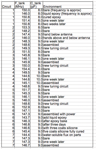
Figure: Tank Resonance Variation. We measure tank frequency relative to the 146.0 MHz calibration frequency of our A3023CT power source.
Liquid epoxy and liquid flux both drop the tank resonance by three or four Megahertz. Cured epoxy does not appear to affect the tank resonance. Each 1-pF we add to the tank capacitance decreases the resonant frequency by 5 MHz.
We take No.6 and load all components and battery. We encapsulate with epoxy and cure. During the process we repeatedly measure the tank resonant frequency. With the epoxy fully cured, the tank resonance is around 0.5 MHz below the value of the bare circuit. It's frequency response is shown below.
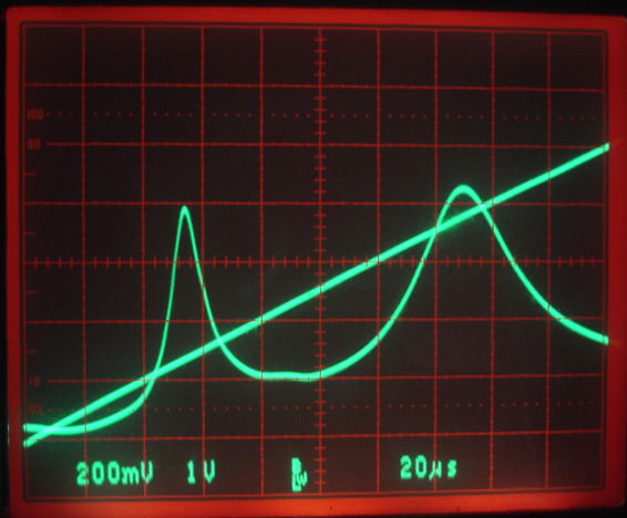
Figure: Response of A3024A Tuning Circuit with Cured Epoxy. Top trace is the VCO tuning voltage, sweeping from 0-5 V in 200 μs. Frequency varies from 116-210 MHz. Bottom trace is the A3024A detector diode output. The first peak is the tank resonance at 146.3 MHz. The second peak is the antenna resonance at around 190 MHz.
We place an active Subcutaneous Transmitter (A3019D) antenna flush up against the A3024A loop antenna. Despite several minutes trying to find a response to the transmitter signal, we conclude that the sensitivity of VR to the A3019D signal is less than 2 mV, and therefore small compared to the 10-mV lamp-switching threshold. We walk around the lab, moving and rotating the encapsulated A3024A with a white LED attached, while sending pulses of power from our booster amplifier. At 20 m we can sometimes pick up a signal. At 1 m it is 100% reliable.
[25-FEB-13] With cured epoxy and three coats of silicone, A3024A No6 has tank resonance at 146.6 MHz, which is close to the 147.3 MHz we measured with only the tuner ciruit loaded.
[27-FEB-13] We find that our A3023CT default frequency has dropped from 146.0 to 145.2. We adjust it to give 146.0 MHz again. We re-measure the tank resonance of all seven of our test circuits. Circuits 1-4 and 7 are within ±0.3 MHz of the values we measured a week ago. No5 has increased by 0.8 MHz. No6, now with five coats of silicone cured over its epoxy encapsulation, has seen its tank resonance drop to 145.5 MHz from 147.1 MHz before assembly and encapsulation.
We clip the extension from No6. We have another encapsulated A3024A, the first one we made with antenna matching, and an encapsulated A3024Y. We tape them to a piece of cardboard and hold this up with a ruler. We hold it with the receiving antenna coils vertical and facing the vertical transmitting antenna. We pulse the antenna power at 10 Hz with 10-ms pulses. The A3024Y turns off at range 40 cm and the A3024As at 200 cm. We now take one A3024 and hold its antenne entirely within our fist, with the antenna oriented coil vertical and facing the vertical transmitting antenna. The No6 A3024A turns off at range 7 m, the original A3024A turns off at range 8 m, and the A3024Y turns off at 2 m. We do the same experiment, but holding only the body of the A3024 with the antenna in air. The No6 A3024A turns off at 8 m, the original A3024A turns of at 8 m, and the A3024Y turns off at 3 m.
Our antenna matching appears to give us a factor of four increase in range when compared to the tank tuner. But we see that holding the body of the implantable lamp with our hand increases the range by a factor of four also. It remains to be seen how well an A3024A will perform when implanted.
Today we observe our A3024As responding to 2.4 GHz wireless transmission from our lap-top at range up to 300 mm and from our mobile phone at range up to 30 mm.
[07-MAR-13] We take out A3023CT No1 and check its output frequency with no TUNE signal applied. We get 145.6 MHz. We take out No2 and get 144.7 MHz. We adust No2 for 146 MHz. We note that No2 delivers an asymmetric waveform, as seen on our oscilloscope.
We use No1 to deliver RF power through various attenuators to our oscilloscope and a bent-wire antenna at the same time. We set up our encapsulated A3024A No0 and No6 in various places at the limit of command frequency reception. We adjust the command frequency so as to find the frequency range over which the lamp turns on. We assume the mid-point of this range is a measure of the tank resonant frequency of the encapsulated transmitter. The table below presents our results.
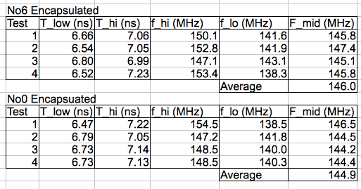
Figure: Upper and Lower Edges of Tank Resonance. We test two encapsulated A3024As and measure upper and lower frequency for which the lamp turns on at the edge of reception range.
The tank resonance of No6, as measured by the frequency sweep, was 145.4 MHz just before we clipped off the extension board. Test 3 on No6 had a broad range. If we take the average mid-range value for the remaining three tests, we get 145.5 MHz. Before encapsulation, No6 had tank resonance 147.3 MHz. It appears that encapsulation causes a 2-MHz drop in tank resonance. We also note that placing body tissue around the antenna drops the tank resonance frequency by up to 3 MHz. Thus the ideal pre-encapsulation tank resonance frequency is around 149 MHz, allowing for 2 MHz drop due to encapsulation and another 1 MHz due to implantation in an animal.
Adding 1.0 pF to the tank circuit drops its resonance by around 5 MHz. With 1-pF capacitors we can place the tank resonant frequency in a 5-MHz window. If we make this window 146-151 MHz, the encapsulated device will have tank resonance 144-149 MHz.
[07-MAR-13] We complete the assembly and testing of five new A3024A circuits. They are numbers 2, 3, 4, 5, and 7. Numbers 0 and 6 we have encapsulated already. Their tank resonant frequencies are 149.3, 150.0, 148.6, 148.6, and 146.7 MHz respectively. We test reception range with our 32-dBm booster amplifier and 1/2-wave antenna. We obtain the same superb performance we did wandering around the laboratory with No0 on 28-JAN-13. Reception is 100% reliable up to 3 m. With the other transmitters, reception is 100% reliable only up to 1 m or 2 m. The tank resonance of No7 is 146.7 MHz, closer to our command frequency than any of the other receivers.
[13-MAR-13] We measure the default frequency of our A3023CT and find it to be 146.0 MHz. We set up a frequency sweep. We re-measure the tank resonance frequency of our five assembled and un-encapsulated A3024As. The following table gives the frequencies before and after we attached the lamp leads, washed with hot water, and baked in the oven for 48 hours at 60°C.
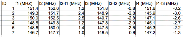
Figure: Tank Resonance Before and After Encapsulation. The No1 matching circuit is already encapsulated in epoxy, and acts as a reference tuner. The f1 measurement was before 48-hr bake. The f2 measurement is after 48-hr bake. The f3 measurement is after we add 0.5 pF capacitors to No2, No3, No4, and No5. The f4 measurement is after encapsulation in epoxy and 24-hr bake.
We add 0.5-pF capacitors to No2 through No5 to adjust downwards their tank resonance frequencies. The 0.5 pF capacitor causes roughly a 2.5 MHz reduction in tank resonant frequency, which is consistent with the 5-MHz drop caused by a 1.0-pF addition.
The resonance No5 is not as sharp as that of the other five circuits. In the past, we have re-built the matching networks of circuits with such behavior, but we choose to leave this circuit as it is.
[14-MAR-13] We build an antenna matching network with 0.5 pF in series with the antenna, and tank circuit 100 nH with 9.0 pF. We obtain a resonant peak twice as high as the one provided by our No1 circuit, at 158 MHz. We add 1.0 pF to the tank and the frequency drops to 152 MHz, but the height of the peak drops by 25% also. We add another 1.0 pF and get 146 MHz but now the peak is no higher than that provided by No1. We replace the tank parallel capacitors with a single 11 pF capacitor. We get resonance at 152 MHz. The peak is the same height as that of No1, but narrower.
[03-JUL-13] We have in hand encapsulated A3024A No6 and No7. We have epoxied circuit No1, and another with no identification number, which we believe to be the one we built on 14-MAR-13. We sent five circuits to ION, all encapsulated, so these must be No0, No2, No3, No4, and No5.
[03-FEB-14] We are constructing seven A3024B, No2.1 through No2.7. We load the tuning circuit and antenna. We use two pre-existing tuned circuits to calibrate our measurement of tank resonant frequency. We have one encapsulated tuner at 151.4 MHz and one bare tuner at 151.7 MHz. We load 9.0 pF for C14 and then add 0.5 pF or 1.0 pF to bring down the tank resonance to within 145-148 MHz.
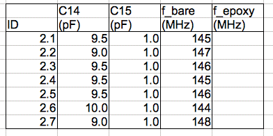
Figure: Tank Resonance of A3024Bs.
Lamp Current
The A3024's lamp power supply consists of an LTC3525-5 5-V boost regulator with a LQH32CN100K53 10-μH, surface-mount inductor and a 10-μF ceramic output capacitor. The input capacitanc is provided by the 1-mF capacitor bank.
[21-DEC-12] The quiescent current of the A3024, when the lamp is off, is of order 2.5 μA. But when the lamp switches on, it draws tens of milliamps from the capacitor bank and the battery. The following calculation shows the relationship between the maximum lamp current and the source resistance of the battery.

Figure: Maximum Lamp Current. Here RB is the battery's source resistance.
We measured the source resistance of a variety of lithium batteries. We connected a 10-Ω resistor across their terminals and measured the voltage across the resistor. This voltage would start at some value and drop slowly. We counted five seconds after connecting the resistor and recorded the voltage. We tested up to twenty batteries of each type. The table below records the average source resistance of the batteries we tested, as we calculate from the voltage across the resistor and the nominal 2.7-V voltage of the lithium cell.
| Type |
Capacity
(mA-hr) |
Diameter
(mm) |
Thickness
(mm) |
Resistance
(Ω) |
| BR1225 | 48 | 12 | 2.5 | 44 |
| BR1632 | 125 | 16 | 3.2 | 50 |
| BR2032 | 190 | 20 | 3.2 | 25 |
| BR2325 | 160 | 23 | 2.5 | 18 |
| BR2330 | 255 | 23 | 3.0 | 26 |
| BR2477 | 1000 | 24 | 7.7 | 18 |
Table: Source Resistance of Various Batteries. Measured five seconds after shorting the battery leads with an ammeter. Data is here.
We see a clear relationship between capacity and volume. But we do not see a clear relationship between resistance and volume. The BR2325 stands out as a battery that delivers exceptionally low source resistance for its volume. A 18-Ω source resistance, combined with the 90% efficiency of the A3024's boost regulator, can provide a continuous current of 18 mA even without a capacitor bank.
We equip our A3024X with a BR2477 battery, two 30-Ω leads, a white LED, part number VLHW4100, and a 10-μF capacitor across the LED, as shown above. We set up our Command Transmitter (A3023CT) with a 3-dB attenuator and rubber ducky antenna attached to its +22-dB output (we do not use the booster amplifier). We turn on the lamp with 1-ms bursts of 146-MHz power. The figure below shows how the lamp voltage, L, and the voltage on the cathode of the LED vary with time during a 1-ms lamp pulse.
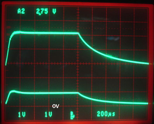
Figure: Lamp Voltage and Lamp Current. Both traces 1 V/div. Bottom trace is voltage on cathode of LED. Top trace is voltage applied to the lamp and its leads combined.
Our 5-V inductive boost regulator produces a lamp voltage of 5.1 V. With the lamp on, the voltage across the 30-Ω cathode lead is 0.90 V, which implies a lamp current of 30 mA. The lamp voltage turns on in 100 μs. It turns off in roughly 400 μs. We have a 10-μF capacitor on the boost regulator output, and another across the LED, and we have 60 Ω combined lead resistance, so we expect a time constant of order 1.2 ms. The LED, however, stops drawing current when its voltage drops below 3 V, so the turn-off will be faster than dicated by a pure RC divider.
The figure below shows how the battery voltage varies during the lamp switching with our A3024X. We see the capacitor bank supplying current for 1 ms, then the battery re-charging the capacitor bank for the remaining 9 ms of the 10-ms flash period.
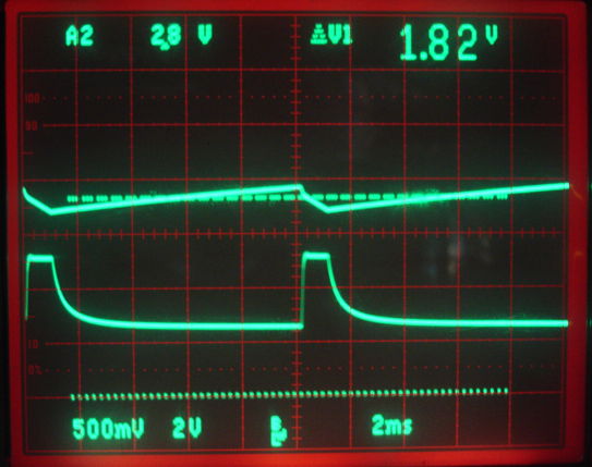
Figure: Battery Voltage and Lamp Voltage. Lower dashed line is 0 V. Top trace battery voltage, 500 mV/div. Bottom trace lamp voltage, 2 V/div. The battery is a BR2477.
Before we start flashing the lamp, our battery voltage is 2.7 V. We start flashing and within a few seconds the average battery voltage drops to 2.2 V. The average battery current, as measured by an ammeter in series with the battery, is 12 mA. After ten minutes, the battery voltage drops to 1.8 V and the average current is 14 mA. We turn off the lamp and the battery voltage rises to 2.4 V in ten seconds and settles to 2.7 V in ten minutes. The battery is not as simple as a voltage source in series with a resistor.
[20-APR-13] Looking closely at the above traces, we see the battery voltage dropping by 50 mV in 100 μs as the boost regulator starts up. This 50 mV drop on a 1-mF capacitor bank suggests that the start-up consumes 50 μC at 500 mA. Such a current is too great for the battery to supply through its internal resistance, so the capacitor bank must be supplying the start-up charge on its own, and we can therefore use the 50-mV drop to estimate the current associated with the start-up. With one light pulse every 10 ms, the start-up consumes 5 mA. If we assume our boost regulator, once it has started up, it 90% efficient, and it is providing 30 mA at 5.1 V from a 1.8-V input, we expect it to draw roughly 90 mA while the lamp is on. With 1-ms pulses every 10 ms we get an average input current of 9 mA. Adding the start-up current to the lamp current we arrive at a total of 14 mA, which is what we observe. We note that the 50-μC charge drawn on start-up is exactly the charge required to raise the voltage on the regulator's 10-μF output capacitor from 0 V to 5 V.
[21-DEC-12] We try a BR1632 battery. After several minutes of 1 ms pulses every 10 ms, the average battery voltage drops to 1.2 V. The lamp continues to flash and the comparator continues to detect the RF power pulses. We stop the flashing and the voltage rises to 2.4 V in ten seconds and 2.7 V in a few minutes.
With a BR1632 battery, we flash for 5 ms every 10 ms and observe the overload of the battery as shown below. The average battery voltage drops to 1 V. The LTC3525-5 boost regulator turns on briefly, turns off, and tries to re-start several times. Its start-up voltage is around 0.9 V, according to its data sheet. As soon as it starts up, the capacitor bank starts to drain and drops below 0.9 V. We note that, even with the 1-V battery voltage, the MC6541 comparator continues to operate. It is specified only down to 1.6 V.
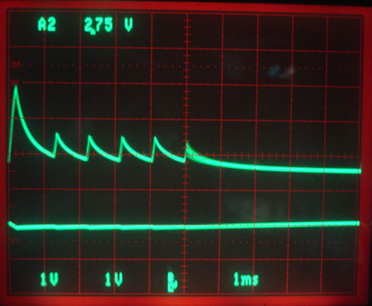
Figure: Battery Voltage and Lamp Voltage. Top trace is lamp voltage. Both traces 1 V/div.
If the comparator produced a HI output when its supply voltage dropped below 1.0 V, we can see how our circuit would get stuck with a battery voltage varying between 0.9 V and 1.1 V as the boost regulator tried repeatedly to turn on the lamp. When we first assembled the circuit, the lamp stayed on of its own accord on two occasions. Since then, we have not been able to reproduce the same effect. But we remain wary that the circuit has this intrinsic flaw: that with the battery overloaded, the comparator will not disable the boost regulator, regardless of the received RF power.
[16-JAN-13] While working with the A3024X today, we observed the lamp stuck on several times as we were loading a battery onto the circuit and shortly afterwards.
[17-JAN-13] We work for an hour with the A3024Y. We modify it several times. We take care to dry the circuit thoroughly after we wash it. We observe no instances of the lamp staying on without RF power.
[31-JAN-13] We load a BR1225 battery onto our A3024A tuned receiver. We attach two 150-mm helical leads. The L− lead has resistance 36 Ω. We solder a C470EZ500 blue LED onto one or our new Head Fixture circuit boards (A302402A) along with a 10-μF capacitor. When the LED flashes, the voltage across the L− lead is 1 V, so the current is 28 mA. We stimulate the A3024A with 1-ms flashes every 10 ms. For ten or twenty seconds, the boost regulator produces full current for the duration of every 1-ms flash. But the battery voltage falls steadly, and after a minute the pulses last only a few hundred microseconds and the battery voltage has dropped to around 1.5 V. When we stop the stimulation, the battery recovers to 2.5 V in half a minute and 2.7 V in a few minutes.
We replace the C470EZ500 LED with an OVLBB4C7, which is also 470-nm blue. We generate 5-ms flashes every 50 ms. After five minutes, we see the following traces of light power and detector voltage. Once again, the boost regulator is aborting the flashes half-way through.
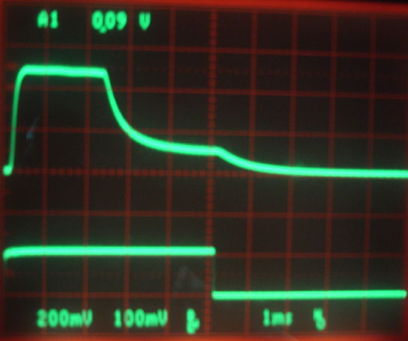
Figure: Aborted Light Flashes. Top trace 100 mV/div is the voltage across a photodiode resistor indicating peak photocurrent of 2.4 mA. The bottom trace 200 mV/div is the detector diode output. The stimulus is 5-ms pulses every 50 ms.
We use a SD445 photodiode and a 100-Ω resistor to obtain the above trace of light power. The unbiased SD445 sensitivity is 0.18 mA/mW at 470 nm, so we conclude the peak power output is 13 mW. The peak current is 25 mA.
Switching Noise
[04-JAN-13] We solder a two-loop 3-cm diameter detection antenna to the A and GND terminals of our A3024X. We load R4, C13 and D2 into the circuit, but not the tuning capacitor C14 nor the tuning inductor L2. We set up our Command Transmitter (A3023CT) with a 3-dB attenuator and rubber ducky antenna attached to its +22-dB output. We do not use the A3023CT's booster amplifier. We load the comparator that detects the presense of radio-frequency power and the boost regulator that powers the lamp.
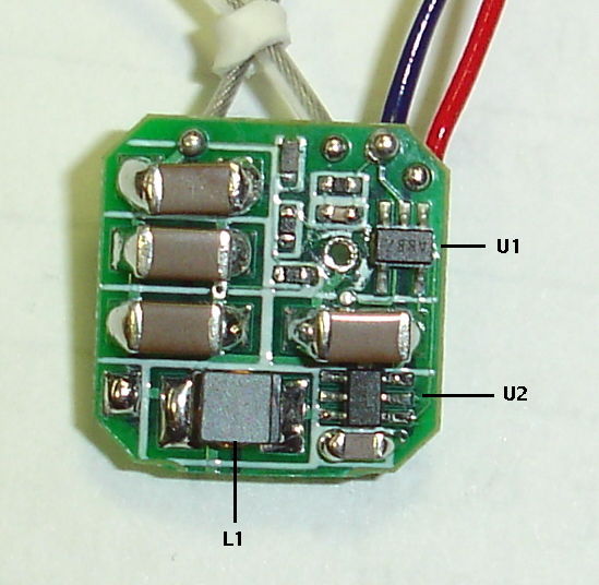
Figure: Comparator Side of the A3024. This is the side that will be exposed. The large components are the 100-μF capacitors of the capacitor bank. The circuit is 12 mm wide.
We attach a battery, as shown here. The figure below shows the RF detector output, VR, during a 1-ms lamp pulse. We see the lamp power turning on when the detector output rises above the 10-mV threshold set by R1, R2, R3, and D4 (see S3024A_1).
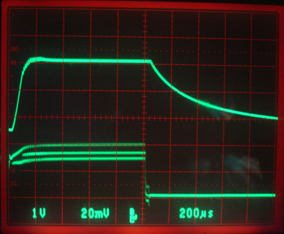
Figure: Detector Output (VR) and Lamp Voltage (L). Top trace is lamp voltage, 1 V/div. Bottom trace detector output, 20 mV/div.
We see on VR a three-level square wave of roughly 10 mV p-p. When we look at the voltage across inductor L1 used by the boost regulator, we see the same square wave, but with peak-to-peak amplitude 5 V. In the lamp voltage, we see a triangle wave that corresponds to current being fed into or drawn out of C11, the boost regulator's output capacitor. The frequency of the square wave is around 500 kHz, which agrees with the LTC3525-5 boost regulator's advertised switching frequency. We can see the square wave more clearly in the close up below.
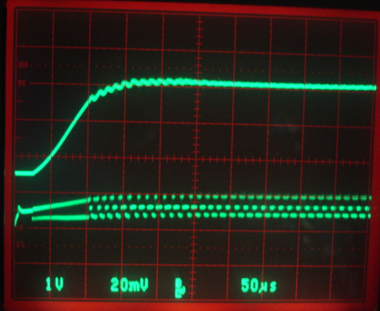
Figure: Detector Output and Lamp Voltage, Close-Up. Top trace is lamp voltage, 1 V/div. Bottom trace detector output, 20 mV/div.
When we disconnect the A3023X battery, the square wave on VR vanishes. We conclude that the square wave on VR is noise from the boost regulator.
[16-JAN-13] With our tuning circuit in place, we turn on power and flash the lamp with an RF signal. The tuning circuit selects 146 MHz at the input of the tuning diode. At the boost regulator frequency of 500 kHz, inductor L2 has impedance 0.3 Ω. We see the same square wave on VR, although only 8 mV p-p.
Optical Power
[14-JAN-13] We measure the power emitted by various LEDs for increasing current. We use the SD445 as our power sensor. You will find its sensitivity in A/W plotted against wavelength here. For 527 nm green light we use 0.25 A/W. For 470-nm blue light we use 0.20 A/W. For white light we use 0.30 A/W, which is the average sensitivity from 450 nm to 650 nm.

Figure: Power Emitted versus Current for Various LEDs.
According to the EZ290 data sheet, the minimum power output of the blue C470EZ290-021 at 20 mA forward current should be 21 mA. According to the calibration of our sample diodes, the power should be at least 27 mW for this particular LED. But we measure only 13 mW. According to the same data sheet and calibration, the green EZ290s should produce at least 11 mW at 20 mA. But we measure only 7 mW. The EZ500 data sheet, meanwhile, specifies a minimum of 40 mW of green light at forward current 150 mA. We see 26 mW at 46 mA, which suggesets of order 85 mW at 150 mA.
[20-FEB-13] We mount all our remaining blue EZ500 and EZ290 sample LEDs and measure their output power at 30 mA forward current. We obtain the measurements tabulated here. We cut three 10-cm lengths of WF300/330/P37 optical fiber and polish both ends. We mount a blue EZ500 on our fiber coupling stage. At 30 mA current it emits 26 mW. We align one end of each fiber with the emitting surface of the LED and measure the power coming out the other end with a photodiode. We invert the fiber to test the other end.
A 400-μm diameter fiber on our 480-μm LED will receive roughly 54% of emitted light. With numerical aperture 0.22 we expect 5% of this light to be trapped within the fiber. Thus we expect 0.7 mW to emerge from the tip. We see 1.5 mW. The same size fiber with numerical aperture 0.37 will trap 15% of light entering, so we expect it to deliver 4.5 mW. With a 300-μm diameter fiber we expect the base to receive 31% of the emitted light, and of this 15% will be trapped. We expect 1.2 mW to emerge. We see 2.4 mW. A 400-μm fiber with numerical aperture 0.37 has 1.8 times the area, so we expect it to deliver 4.3 mW.
[27-FEB-13] We now have three lengths each of four different types of optical fiber, polished at both ends. We measure numerical aperture in the following way. We make marks 100 mm apart on a piece of paper. We mount the fiber over an LED. We hold the sheet of paper in front of the light-emitting tip of the fiber, perpendicular to the fiber axis. We move the paper away until the cone of light emitted by the fiber fills our 100 mm space. We measure the distance to the paper from the fiber tip. In the case of the WF300/330/P37, the paper is 110 mm away. The emitted light cone subtends an angle ±24.4° with the fiber axis. Its numerical aperture is 0.41, larger than its specified 0.37. We have a new spool of WF400/440/P37, and its numerical aperture is 0.37 when we measure it. We have two other 400-μm fibers with numerical aperture 0.25 and 0.24. We fit these fibers and align them over an LED and measure power out of the tip with a photodiode. We obtain the results tabulated here, in which we see the fraction of power captured by various fibers and for our 480-μ square C460EZ500 and 290-μm square C470EZ290. We used an unbiased SD445 photodiode to measure power output from the LED and the fiber tip. We assumed sensitivity 0.20 mA/mW for both wavelengths.
In the above table, we calculate the theoretical capture fraction in two steps. First we estimate the fraction of light that will enter the fiber, based upon the area of the fiber and the area of the LED. Second we apply our cosine-distribution solution to the capture efficiency of a fiber of known numerical aperture, which we present here.
We examine the disagreement between the theoretical and observed capture fractions. In the case of the 400-μm fiber over the 290-μm square LED, we assume all the LED's light enters the fiber. The fiber is larger than the diagonal of the square, and pressed within 50 μm of the LED surface by pressing down the bond wire. In this case we observe 15% capture fraction and calculate 14%. This result suggests that our calculation based upon the fiber numerical aperture is accurate. The slight difference in the two might be explained by the slight deviation from the cosine distribution seen in the measured emission pattern of the EZ500, which shows the light being slightly more concentrated in the forward direction. At 22.5°, for example, the cosine distribution suggests 92% intensity, while the measured intensity is 90%. At 45°, the cosine distribution is 0.71 while the measured is 0.67.
In the case of the 300-μm fiber over the 480-μm LED, we assume that only 30% of the light will enter the fiber. But our observed capture fraction is 9% and our calculation is 5%. This result suggests that closer to 60% of the light emitted by the 480-μm LED is entering the 300-μm diameter of the fiber. The light emitted by the 480-μm square area is concentrated towards the center.
If we now place a 400-μm fiber with NA = 0.37, NA = 0.25, or NA = 0.22, on the 480-μm square LED, the measured capture fraction is roughly 1.6 times the calculated fraction. This result is also consistent with concentration of light towards the center of the light-emitting area.
Our 300-μ NA = 0.41 fiber's capture fraction with the 290-μm LED is 17%, while that of our 400-μm, NA = 0.37 fiber is 15%. If we assume that all the light from the LED enters both fibers, then the difference in capture fraction is consistent with our calculation due to numerical aperture. This suggests that the light emitted by the 290-μm LED is also concentrated towards the center, so that all of the light enters the 300-μm fiber.
We conclude that our numerical aperture calculation, which assumes a cosine distribution of light emission by the LED, is accurate, but our assumption of uniform distribution of light across the LED is not. The light is concentrated towards the center of the emitting area. Thus we are able to obtain almost double the capture fraction that we would with uniform light distribution.
With the 300-μm, NA = 0.41 fiber on the EZ290 we get 17% of the light emitted by the LED emerging from the tip of our fiber. If we could obtain an C470EZ290 that emitted 40 mW for 30 mA current, as specified by the data sheet, we would obtain 6.8 mW at the fiber tip. As it is, our EZ290s are producing only 17 mW at 30 mA, so we see only 3.0 mW. We do not know why our EZ290s are performing so poorly. The are emitting less than half the light we expect from the calibration sheet supplied with our samples. In the case of the EZ500, the LEDs produce 25 mW for 30 mA current, and we get 11% capture efficiency with our 400μm, NA = 0.37 fiber. So we obtain 2.6 mW at the fiber tip.
As things stand today, we can obtain roughly 3 mW with both the EZ290 and the EZ500, using our high numerical aperture 300-μm and 400-μm fibers respectively.
[06-MAR-13] Measure power emerging from a 7-mm taper glued to a blue EZ290 that emits 16.4 mW at 30 mA. We placed our 10 mm × 10 mm photodiode in five different locations around the fiber tip to make five faces of a cube with the tip at the cube center. Because we place the photodiode with only ±10% distance accuracy, we expect this measurement to be good to only ±20%. We measure a total photocurrent of 450 μA, which correspods to 2.25 mW, or 14% capture fraction.
[20-MAR-13] The following calculation shows how the refractive index of the fiber core, cladding, glue, and surrounding air affect the numerical aperture of the fiber base.

Figure: Calculation of Numerical Aperture for Various Cladding Environments.
In Fiber-Cladding Adhesive we describe our plans to quadruple the power emitted by replacing our clear epoxy with a UV-cured adhesive of refractive index 1.32.
[01-APR-13] We receive three types of the Luxeon Z die LED from Philips Lumileds. The light-emitting area of these devices is roughly 1 mm square. The die has pads on the bottom for soldering, so requires no wire-bonding. We run 30 mA through the LXZ1-PB01, a 470-nm blue LED. We get 5.8 mA photodiode current, or 29 mW total power. The LXZ1-PE01, a 505-nm cyan LED gives us photocurrent 5.2 mA, or 23 mW (0.23 mA/mW at 505 nm). The LXZ1-PL01 is a 590-nm amber LED that gives us photocurrent 1.4 mA, or 4.2 mW (0.33 mA/mW at 590 nm).
[08-APR-13] We receive 2363 of C460EZ500-0214-2, with average wavelength 459.5 nm and minimum power output at 150 mA of 150 mW. The LED dies arrive in between two plastic sheets, as you can see here. The manufacturer's calibration sheet is here. The calibration suggests that we can expect a total of 150 mW of blue light for a forward current of 150 mA. We solder one LED die to a circuit board and make contact with its cathode by means of a stainless steel whisker.
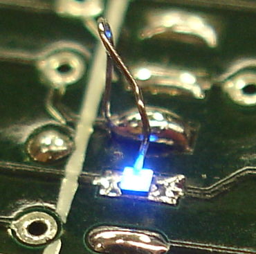
Figure: EZ500 Mounted with Stainless Steel Whisker.
We hold our 10-mm square photodiode 2.1 mm from the emitting surface (the height of the steel whisker) and measure 4.4 mA of photocurrent, which is 22 mW of optical power. If we assume a cosin distribution of light from the LED, we expect to get roughly 85% of the emitted light incident upon our photodiode. We estimate that our steel whisker shadows roughly 5% of the light. So the 22 mW on our photodiode suggests almost 28 mW of total output power. This measurement is consistent with the Cree calibration of around 30 mW for 30 mA.
[26-APR-13] We receive 25 C460EZ500 LED dies from our new batch mounted in 3-mm QFN-8 packages. We measure the light power emitted by one such part with a photodiode. We bias the photodiode with 0 V and with 9 V. The photocurrent is 6% higher with bias. We decide to use the biased photocurrent as our measurement of power. We convert photocurrent into total radiant power with 0.20 mA/mW for 470 nm and 0.19 mA/mW for 460 nm. At 30.0 mA forward current the C460EZ500 emits 27.7 mW and the LXZ1PB01 emits 29.0 mW. With no bias on the photodiode we measured 26.6 mW and 27.6 mW respectively using the same responsivity. Thus we propose that the responsivity of the un-biased photodiode is closer to 0.182 for 460-nm light and 0.191 mA/mW at 470 nm.
We polish both ends of a 390-μm diameter, 50-mm long, F2-core fiber, and clean it with acetone. We lower it onto the EZ500. We run 30.0 mA through the diode and measure 10.1 mW coming out of the tip. We note light escaping from the sides of the fiber. We coat the fiber in place, axis vertical, with NO13685 clear adhesive. The coating appears effective when we first apply it, but light begins to leak out even as we cure it. We apply several coats, and the base of the fiber looks like it has bubbles under it. We cure, apply NO68 adhesive and cure that too. But now there is only 4.5 mW coming out of the end of the fiber.
[02-MAY-13] We mounta another C460EZ500. It emits 27 mW at 30 mA. We cut and polish an 80-mm long, F2-core fiber and place it over the LED with our alignment fixture. We place the fiber base just beside the cathode pad, so that the fiber is roughly 100 μm off-center. We see 3.8 mW coming out of the end. We center the fiber so that it smashes down the cathode bond wire. We see 9.1 mW at the far end. We coat the fiber with black epoxy to make sure that we are seeing only the light captured by the fiber core and its cladding. We see 7.7 mW. We get almost twice the power out of the fiber tip by centering the fiber on the LED die.
[03-MAY-13] We coated our 80-mm fiber with epoxy and left it to cure overnight in a horizontal position. Below is a close-up of the drops of epoxy formed by surface tension. We see that there remains a coating of epoxy between the lumps.

Figure: Drops of Black Epoxy on A 390-μm Fiber. The glue cured with the fiber axis horizontal.
We polish the end of this fiber again, to remove any epoxy that might have covered the tips, and place over our C460EZ500. With the fiber base centered as best we can on the LED die, we obtain 8.2 mW out of the upper end, which is a capture efficiency of 30%, a new record.
[07-MAY-13] We work with EZ290 green LEDs and our high-index fibers, trying out various coatings. We describe our experiences in Polishing, Cleaning, and Curing. We decide it's not worth trying to coat the fibers with adhesive. Better to get a higher-index fiber.
[08-MAY-13] With our monochrome ICX424 image sensor we obtain the following image of the EZ500 with 80 mA forward current. We placed two neutral density filters between the LED and the camera, to stop saturation of the image sensor pixels. The total optical density was 3.0, for 0.1% transmission.

Figure: Distribution of Light Across EZ500 Surface.
Taking the background intensity as 0.0, the peak intensity in the center is 135 counts. Along the edges, the intensity is 77 counts. Thus we see that the central region is almost twice as bright as the peripheral regions.
[10-MAY-13] We cut 225 sections of our NA = 0.66 fiber, taking the sections at random from all the coils of fiber in our box. We measure their diameters at one point each with a micrometer. Our resolution in measuring diameter is 3 μm with our micrometer. We obtain the following histogram.

Figure: Distribution of Diameter Among Samples.
The average diameter is 405 μm with standard deviation 12 μm. The minimum is 370 μm and the maximum is 440 μm. We measure diameter along the length of a selection of fibers and obtain the following plots.

Figure: Changes in Diameter With Position.
The most rapid change in diameter we observe is 30 μm in 100 mm. Along an 8-mm ISL fiber, we would see no more than a 0.6% change in diameter. With the help of a program we calculate the fraction of EZ500 light that will enter the core of a fiber as a function of outer diameter. We assume the core takes up 87% of the area. We calculate the fraction of EZ500 light that will reach the far end of the fiber for NA = 0.66 and NA = 0.86.

Figure: Capture Efficiency versus Diameter. We show the fraction of light incident upon the fiber base, the fraction that reaches the other end for NA = 0.66, and for NA = 0.86. We assume 87% of the fiber is high-index core.
We see that 30% capture efficiency we observed with our existing NA = 0.66 fiber is consistent with an outer diameter of 450 μm, and 27% with 420 μm.
[28-JUN-13] We received our Higher Index Fiber at the end of March. The core is a glass that Fiberoptics Technology calls TD5. The numerical aperture is supposed to be 1.72. We measured the diameter of 178 sections of fiber and obtained an average of 411 μm and a range 390-440 μm. Today we found a section with diameter 450 μm and made a 80-mm length. We polished both ends and examined through the fiberscope. The surfaces are near perfect after polishing with 1-μm diamond grit.
We apply 30 mA to a 460-nm EZ500 and obtain 32 mW output (5.8 mA in our SD445 photodiode, sensitivity 0.18 mA/mW at 460 nm). We lower our fiber onto the LED. We apply NO68 UV-curing adhesive to the base of the fiber. We cure for five minutes in UV light. We measure 9.6 mW at the tip. We pull the fiber out of the semi-cured adhesive and measure 25 mW total power from the LED.
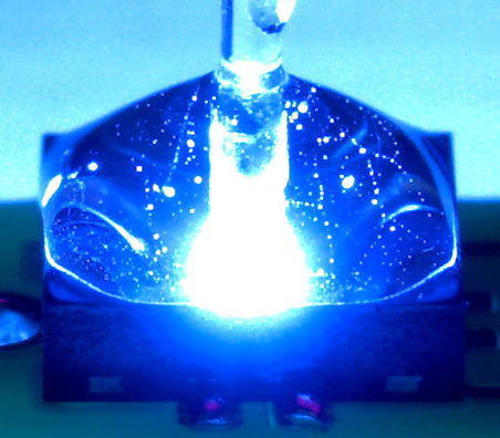
Figure: Bubbles in the UV Adhesive During Curing in UV Light. The LED current is 30 mA.
We try another EZ500. With 30 mA it emits 31 mW. We lower our fiber into place, with 20-mm of its length covered with nail polish. WE measure 16 mW at the fiber tip, which is 51% of the light emitted by the LED. We note that the LED is tilted up off the package floor by the bond wire beneath it, at an angle of about 10°. We apply E-30CL epoxy. We tried to remove bubbles from the hand-mixed epoxy with a vacuum chamber, but the result was very tiny bubbles. After applying the glue, the power at the tip is 9.1 mW. We remove the fiber and measure only 24 mW total output power. We soak in ethanol to remove epoxy and now observe 30 mW. We wash some more and get 27 mW.
[24-OCT-13] Yesterday glued a 146-mm higher-index fiber (NA = 0.86) to a C460EZ500. We used a mixing nozzle and a syringe to apply the glue. There were no bubbles. But we were mystified by loss of power at the top end of a 146-mm fiber when we applied the glue. Today the epoxy is cured. We apply 30 mA to the LED and obtain 8.2 mW at the top end. Yesterday we measured the total power output at 30 mA to be 25.7 mW. Our capture efficiency appears to be 32%. We apply clear epoxy to 30 mm of the fiber, towards the top. Power at the tip remains 8.2 mW. We cut back the fiber from 146 mm to 30 mm and polish the end. We apply 30 mA and get 10.6 mW at the tip. The result is shown below.

Figure: A 30-mm Higher-Index Fiber. Click on image for higher resolution. The base is glued to a C460EZ500. The tip is polished. The conical angle of the output is around &plumns;60°, which is consistent with a numerical aperture of 0.86.
The T5 glass used in this fiber is proprietory. The fiber manufacturer told us the T5 glass was "very yellow", which we take to mean that it absorbs blue light. Suppose the T5 glass is similar to Schott P-SF69 glass, which also has refractive index 1.72. In that case, transmission over 10 mm is 98.5%, which means we will lose 20% of our light going 146 mm and 4.5% over 30 mm. If the T5 glass introduces loss η after 10 mm, and the power coupled into our fiber at the base is P, then Pη3 = 10.6 mW and Pη14.6 = 8.2 mW. From this we conclude that 11.3 mW is being coupled into the fiber base and transmission over 10 mm is 97.8%. Coupling of 11.3 mW out of 25.7 mW is 44%. It may be that the LED is producing 29 mW today, in which case coupling efficiency is 39%, matching our calculation. See Yellow Glass for another report.

Figure: Taper in 410-μm Higher-Index Fiber. Blue 460-nm light. Taper is 2.0 mm long.
[28-OCT-13] We take a new C460EZ500. It's output power at 30 mA forward current is 27 mW (4.85 mA photocurrent through unbiased photodiode). We glue with five-minute epoxy a fiber 40-mm long with a polished base and tapered top. This fiber looks to be about 410 μm in diameter. We allow the glue to cure. We press our 10 × 10 mm2 photodiode against the side of the fiber, with the taper at the center of the photodiode. In this way, we expect to get the light emitted by the taper outside ±20° from the axis, and within a ±80° slice in the radial direction. We see 3.7 mW (0.67 mW photocurrent). We hold the photodiode 15 mm from the top of the taper, and perpendicular to the fiber axis. We now receive most of the light within ±20° of the axis. We see 1.1 mW (0.2 mA photocurrent). Multiplying the first measurement by 2×9/8 and adding the second, we arrive at 9.4 mW total emission from the taper. Assuming 2.2% loss per 10 mm, the power entering the base of the fiber should be 10.3 mW, which is 38% of 27 mW.
[03-NOV-13] Last week, Mr. Collins sent us the following photograph of three tapers he made consecutively on his tapering machine.

Figure: Three Tapers Made Consecutively. Graduations on the ruler are 0.5 mm.
From the base to the tip of the taper is a little over 2.5 mm. These are made with our higher-index fiber, core made of T5 glass and cladding of silica.
[14-FEB-14] We load leads and batteries onto seven A3024B assemblies. No2.2, 2.3, 2.4, and 2.5 we equip with the small battery and 50-mm unstretched leads. No2.1, 2.6, and 2.7 we equip with the large battery and 100-mm stretched leads. At the tip of all leads we solder a 300-μm diameter pin. The combined resistance of the leads is 55 Ω on average (see here). With 2.8-V forward voltage on the LEDs and 5.05 V boost regulator output, we expect an average of 41 mA lamp current. We charge all the batteries and glue them to their circuit boards. During this process, we damage No2.6. Two hours of work burning off epoxy does not solve the problem, so we discard. We coat in epoxy twice, then dip in silicone twice and leave to cure.
[19-FEB-14] We clip the leads of No2.4 at a point 5-mm from their base, strip 2 mm of insulation, and solder stretched leads to the exposed steel helix. The resulting leads are 50 mm long. The resistance of the wire we added was 12.5 Ω for L+ and L−. The resistance of the 3 mm of the unstretched leads is around 3.0 Ω. Add another 1 Ω for the resistor on the head fixture, and we have a total resitance of around 29 Ω. The forward voltage drop of our C460EZ500s is 2.88 V at 42 mA, so should be around 3.00 V at 70 mA. With a 5.05-V lamp voltage, we are hoping for around 70 mA. Head fixture No2.4 has 41.2% coupling and the LED emits 55.3 mW at 70 mA, so if we combine A3024B No2.4 with A3024HFB-B No2.4, we should get 22.8 mW at the tip. At the very least we expect 20 mW.
Head Fixture
[04-MAR-13] We assemble a head fixture out of a cut-off 300-um fiber glued to an EZ500 LED. We solder 2.1-mm long gold-plated pins (Mill-Max 4353-0-00-15-00-00-33-0) to the leads of our original A3024A. To the head fixture circuit board, A302402A, we solder two sockets (Mill-Max 4428-0-43-15-04-14-10-0). We use clear five-minute epoxy to fix a silica guide cannula (Plastics One C313GS-4-FS-SP) to the A302402A.

Figure: Prototype Head Fixture. (1) L+ lead from A3024A. (2) L− connector pin. (3) L− connector socket (L+ socket is beneath). (4) 300-μm fiber coupled to EZ500 LED. (5) Silica Guide Cannula. (6) 4-mm pedestal. (7) Smoothing capacitor. (8) is the A302402A circuit board, after clipping off its mounting extension.
The head fixture is supposed to look like the one we proposed in Fiber and Cannula. We have added connectors to the head fixture circuit board, so the lamp controller and the head fixture may be separated. This prototype does not provide an EEG electrode at the fiber tip.
[14-MAR-14] We assemble seven Head Fixtures (A3024HF). We use five-minute epoxy to glue the guide cannula to the head fixture circuit board. We cover this epoxy with black potting epoxy to mask the light escaping from the base of the fiber.
We omit the 10-μF capacitor we had planned to put on the head fixture circuit board. When the A3024A is switching the lamp on and off, the lamp voltage varies from 3 V to 5 V in the off and on states respectively. The 10-μF capacitor on the output of the 5-V boost regulator in the A3024A circuit maintains the lamp voltage at just below the forward voltage drop of the LED. We do not see the rapid rise from 0 V to 3 V at turn-on that the 10-μF capacitor on the head fixture was suppoed to mitigate. Thus we have no need of the head fixture capacitor.
The black epoxy, by masking the light leaking from the LED, makes it easier for us to measure the optical power emerging from the fiber tip. We hold our photodiode 5 mm from the taper on all four sides and above. We measure a total of between 2 mW and 3.5 mW, but we believe our error to be of order ±0.5 mW.
Another purpose of the black epoxy is to stop the animal being subjected to a bright, visible light that, by being visible, might affect its behavior and so corrupt our optogenetics experiment. But a disadvantage of the black epoxy during development is that we will may see no evidence of the response of an implanted lamp.
We insert dummy cannulas in each head fixture and arrange all seven on double-sided sticky tape in a box. Later, when we pack them up, we will put each of them in a petri dish on a piece of sticky-tape, and hope that this protects the delicate device during transportation.
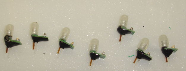
Figure: Set of Head Fixtures (A3024HF).
[15-MAR-13] We assemble two test lamps using our white VLHW4100 LED and the tiny sockets. We arrange the sockets to mimic the head fixtures, and color the LED leads to match the color of the wires on the implantable lamps.

Figure: Test Lamps for Use with A3024A.
When placing the A3024A in a bag, we realise that we must take some precaution against its leads coming into contact. If they remain in contact, and the lamp is stimulated frequently by some source of RF, the current flowing through the contacts will exhaust the battery. We wrap a post-it note around one of the leads before placing the device in a bag.
[29-APR-13] Here is a drawing of the tapered fiber. We are sending out this drawing to sapphire manufacturers, hoping they can make the entire thing with optical finish out of sapphire with refractive index 1.73.
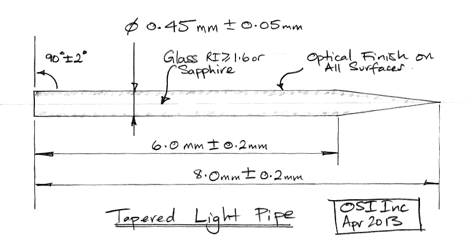
Figure: Proposed Sapphire Light Pipe.
If we coat sapphire with epoxy of index 1.50, we will obtain numerical aperture 0.86, which will capture 75% of the light entering its base from an LED. With diameter 450-μm over our EZ500 die, we will have 69% of the light entering the base. The net coupling efficiency to the fiber tip will be 52%, even if there is no concentration of light towards the LED center.
[13-DEC-13] We have a new Head Fixture, the A3024HFB (following the A3024HF). The new fixture is built upon the A302402B circuit board. The QFN-8 footprint is improved. Instead of a hole for the guide cannula we have a notch. We provide a MOLEX-2 plug socket for use during assembly, and two miniature sockets for use during implantation. Before delivery, we will clip off the extension with the MOLEX-2 plug. We assemble nine boards and measure the output power of the LEDs at various currents.

Figure: C460EZ500 Output Power at Various Currents. We give diameter of fiber we later glued to the LED and the coupling efficiency. The coupling efficiency is the fraction of light emitted at 30 mA that emerges from the fiber tip. NOTE: We later find that coupling efficiency of No2.2 is in fact
The LED in a tenth assembly emits 26.7 mW at 30 mW. This one we glue to an 8-mm tapered higher-index fiber. We discuss the resulting assembly in New Head Fixture. The head fixture with blue C460EZ500 LED will be the A3024HFB-B, and with green C527EZ500 LED will be A3024HFB-G.

Figure: Higher Index Glass Fiber on New Head Fixture. Guide cannula not yet attached. Power emitted by the tip is roughly 10 mW at 30 mA LED current. The LED produces 26.7 mW at this current. Assembly A3024HFB-B, No2.10.
Not yet installed in the A3024HFB-B shown above is the guide cannula, which will have a 9-mm silica tube that we will attach to the base of the taper and to the side of the LED, in the notch provided by the circuit board. Power to the LED enters at the MOLEX-2 plug or the miniature sockets. In series with the anode of the LED we have a P0805 resistor. We plan to use this resistor to set the LED current given the resistance of the leads from the implantable lamp.
[18-DEC-13] We measure the power output of A3024HFB-B No2.9 in two ways. We place our photodiode in five positions around the taper so as to make a virtual box of photodiode that absorbs all light it emits. By this means, we measure total power 10.8 mW. We place our SD445 photodiode up against the taper and at an angle, like this. We estimate that we will get all the light emitted by the taper within a 160° angle in the horizontal plane and from −45° to +90° in a vertical plane. There is very little light emitted downwards at 45°, so we estimate that we are receiving 4/9 of the light emitted by the taper (we made the same argument on 28-OCT-13). By this means we obtain an estimate of 10.8 mW also. We will use this latter method in the future.
[09-JAN-13] We receive 9-mm guide cannulas from Plastics One, part number C313GS-4-FS-SP. Our plan is to glue the tip of the guide cannula to the base of the taper, so that they are joined, in contrast to our original head fixture design, where the guide cannula was pointing towards the taper but not attached to it.
The 9-mm guide is too long for head fixture A3024HFB-B No2.2, so we sand it down with 15-μm grit paper until it looks right. We glue it in place with five-minute epoxy. We manage to avoid blocking the guide cannula with glue, nor do we see any glue on the taper. The guide cannula and the tapered fiber are shown below, immersed in water, and emitting blue light.

Figure: Head Fixture No2.2. We sanded the 9-mm guide cannula down to a length of roughly 8 mm so that its tip would be adjacent to the base of the taper. The outer diameter of the fiber is 450 μm and of the guide is 700 μm. The misty blue light in the upper foreground is an artifact of the plastic petri dish between the water and our camera.
There are three ways to define the base of the taper. One is the physical base, where we first observe curvature of the outer glass. This is the definition we used when gluing the guide in place. We also have the point along the taper that first emits light when the taper is in air, and when the taper is in water. The taper emits light earlier in water than in air. The brain is mostly water, so we immerse the taper in water for the photograph above. We see that the guide cannula ends roughly 300 μm before the emission of light.
[17-JAN-14] We attach a 460-μm diameter taper to No2.3. We apply glue. We place in the oven at 60°C to cure. When we take it out, we find that the base of the taper is about 100 μm off-center. Output power is 9.5 mW at 30 mA current. As we are masking the base of the taper, we break it off and we have to discard both taper and LED. We attach a 460-μm taper to No2.6 and leave to cure at room temperature.
[21-JAN-14] No2.6 is cured. The base of the fiber is off-center in the direction perpendicular to the bond wires by roughly 100 μm. Using this method we measure the taper output power to be 10.4 mW at 30.4 mA forward current.
[22-JAN-14] We glued a 460-μm taper to No2.7 yesterday. The base of the fiber is well-centered, but the glue is still tacky. We throw the cartridge away. Power output from the tip is 10.4 mW at 30 mA. We glue a 440-μm taper to No2.5.
[23-JAN-14] No2.5 emits 10.4 mW at 30 mA, despite having a 440-μm fiber rather than a 460-μm fiber. We glue a 440-μm fiber to No2.8.
[24-JAN-14] When trying to remove No2.8 from our clamp, we snap off the fiber. We glue a 440-μm fiber to No2.4. Before we apply glue, we measure 16 mW being emitted in the forward direction from the fiber tip at 30 mA LED current. We take out No2.6 and measure its power output with 30 mA. We mask the LED with aluminum foil. With the this method we get 0.83 mA of photocurrent, so total power is 9/4×0.83/0.18 = 10.4 mW. With the fiber perpendicular to the photodiode and the tip touching the photodiode, we get 1.3 mA photocurrent, or 7.3 mW incident on the photodiode. Given that the photodiode extends for 5 mm from the tip, and the light emission takes place along a 1-mm length, we see that everything emitted within ±84° of the fiber axis is incident upon the photodiode. The missing 3 mW must be emitted at an angle greater than ±84°.
[27-JAN-14] The taper of No2.4 emits 11.0 mW at 30 mA forward current, for coupling efficiency 41%. We try to polish our photodiode, whose acrylic glass is scratched by fiber tips. We succeed only in making it a mess of smaller scratches. Its sensitivity remains the same. We snap one of its leads off, so take out a new photodiode. Its sensitivity is the same.
We mount a guide cannula in our fiber clamp and use our three-axis stage to place the tip of the guide cannula 450 μm from the tip of tapera No2.5. We glue with five-minute epoxy. We take this photograph of the head fixture in water. The light-emitting length of the taper in water is 1000 μm.
[30-JAN-14] Another A3024HFB-B for taper No2.4, see here for photograph in air. The cannula ends 900 μm from the tip of the taper.
[31-JAN-14] Another A3024HFB-B for taper No2.7, photograph below shows how light-emitting length of taper is shorter in air than in water.
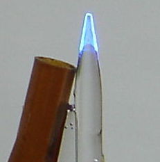
Figure: Head Fixture No2.7 in Air. Cannula ends 1000 μm from taper tip. Light-emitting length in air is 700 μm.
The light-emitting length in water is 1000 μm and in air is 700 μm. We expect the light to escape earlier in water because water's refractive index is higher than that of air.
[06-FEB-14] We test the miniature sockets on our head fixtures, and take photographs of No2.9, No2.10, and No2.6. No2.6 is damaged: the tip of the guide cannula has broken off. The tip of the cannula was not glued directly to the fiber, the glue having sunk down to the base of the cannula and LED before it cured. In the future, we must ensure that the tip of the cannula is protected by glue. We replace the guide cannula by hand, and the result is satisfactory, as shown in the No2.6 photograph. No2.10 is dirty: there is residue from electrical tape we used to mask the LED during power measurement. This residue is trapped under the glue. We switched to using aluminum foil after we realised the problem with electrical tape, and found aluminum foil to be more effective and convenient.
[11-FEB-14] We have five C527EZ500 green LEDs mounted on A302402B circuit boards. These are A3024HFB-G assemblies. We measure their power output with an unbiased SD445 photodiode at various currents. We use 0.23 A/W for the photodiode sensitivity.

Figure: C527EZ500 Output Power at Various Currents. We give diameter of fiber we later glued to the LED and the coupling efficiency. The coupling efficiency is the fraction of light emitted at 30 mA that emerges from the fiber tip.
[14-FEB-14] We have guide cannulas on head fixtures No2.11 and No2.12. Coupling efficiency is around 39%.
Battery Life
[04-JAN-13] The inactive quiescent current of our A3024X (VR is below threshold, the comparator asserts !ON, and the boost regulator is disabled) is 2.5 μA. We have to wait a while to see this current because the capacitor bank must fill up and the battery must settle down after supplying the capacitor bank charge before the current from the battery, which is what we are measuring, is equal to the current consumed by the comparator, resistive divider, and the disabled boost regulator. With a 48 mA-hr battery, this gives us a shelf life of 27 months.
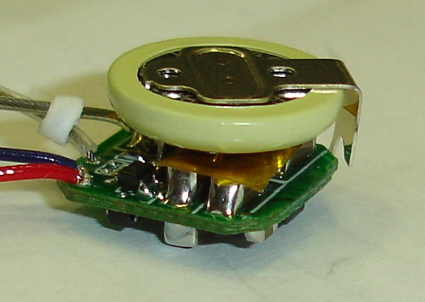
Figure: The A3024 with BR1225 Battery. The large components on both sides of the board are 100-μF capacitors, ten in all to make a 1-mF capacitor ban. Note the insulating orange kapton tape between the battery and the capacitor bank. We eliminate this insulator in later versions.
The volume of the capacitor bank, which consists of 10 P1206 packages, is approximately the same as that of the battery.
Our A3024X provides 30 mA to its white LED through to 30-Ω steel leads. With 1-ms pulses every 10 ms, average lamp current is 3 mA and average battery current is 13.9 mA. As we discuss in our Conceptual Design, we assume the effective capacity of a primary lithium battery for a current of tens of milliamps is half its capacity for a current of tens of microamps. Thus a 48-mA-hr battery will give us 24 mA-hr capacity, and at 13.9 mA this will give us 1.7 hours of lamp life.
[15-MAR-13] We have been using our No0 A3024A since we first constructed it at the end of January. It still provides full-power to its LED. The LED has been flashed with 10% duty cycle for roughly 1 hour so far.
[20-APR-13] We consider the use of lithium-ion rechargeable batteries for the Implantable Lamp, see Lithium-Ion Batteries. We order several types of lithium-ion batteries to try out.
[29-APR-13] We experiment with two types of lithium-ion battery. One is the PP031012AB, with nominal capacity 19 mA-hr. The other is the 382030 with nominal capacity 160 mA-hr. The small one we consider suitable for implantation in mice, and the larger for implantation in rats.
We discharge both batteries with resistors. We charge a small and a large battery by the rapid-charge procedure specified by their data sheets. We supply 10 mA to the small battery and 150 mA to the large battery until their voltages reach 4.3 V, then we apply constant voltage of 4.3 V until the battery current drops to 10% of the rapid charge current. After two hours, both batteries appear to be fully charge. We discharge them with resistors. The graph below shows the small battery discharging through a 200-Ω resistor (A) and the large battery discharging through a 40-Ω resistor (B).

Figure: Charging and Discharging Lithium-Ion batteries. Lines A and B showing the discharge of the small battery through 200 Ω and the large battery through 40 Ω. Lines C and D show the small and large battery charging up to 4.3 V. Lines E and F another discharge with the same resistors. Line G is the large battery discharging through 20 Ω, and H is discharging through 10 Ω.
At 3.7 V the discharge currents (A and B) are 18 mA and 92 mA respectively. While discharging to 3.0 V, the small battery delivers 20 mA-hr and the large one delivers 160 mA-hr. The small battery discharges to 0.0 V through its load resistor, but the large battery is equipped with a protection circuit that disconnects it from the load when the battery voltage drops below 3.0 V, so it does not discharge below 3.0 V.
We recharge at the recommended rate (C and D) and discharge through the same resistors (E and F). The large battery provides 162 mA-hr but the small battery provides only 11 mA-hr. We believe the small battery has been damaged by its complete discharge to 0.0 V. We re-charge the large battery and discharge it through 20 Ω (G). At 3.7 V, the discharge current is 185 mA. The battery provides 148 mA-hr. We re-charge and discharge through 10 Ω (H). At 3.7 V, the discharge current is now 370 mA and the battery provides us with 130 mA-hr.
Lithium-ion battery data denote the nominal capacity of a battery in mA-hr with the letter C. For our large battery, C = 160, so the nominal capacity is 160 mA-hr. The rapid charge current is 0.5C mA = 80 mA. The standard discharge current is also 0.5C mA. The maximum discharge current is 1.0C = 160 mA. The same ratios apply to the smaller battery, for which C = 19. The rapid charge current is 9 mA and the standard discharge current is 9 mA, while the maximum discharge current is 19 mA.
When we charge at 0.5C mA, we get capacity 1.0C mA-hr. But when we charge at C mA, we get only 0.5C mA-hr. If we want full capacity from these batteries, we must take two hours to charge them. Assuming we charge the battery fully, we get capacity C mA-hr when we discharge at 0.5C. When we discharge at 1.0C, which is the maximum recommended discharge current, capacity drops to 0.9C mA-hr. At 2.0C the capacity drops to 0.8C mA-hr. If we allow the battery to discharge completely to 0.0 V, it loses over half its capacity.
[10-FEB-14] We have seven A3024B circuits. They are No2.1 through 2.7. The following table gives current consumption in various states of assembly and stimulation, as measured with a 3.6-V power supply.

Figure: Current Consumption of A3024Bs. We supply the circuit with 3.6 V. We start without the boost converter (U2). The 100 Hz is 100 of 5-ms command pulses per second. When we connect the lamp, 42 mA flows through it. We flash it continuously (100%) or for 1 ms every 10 ms (10%). Eventually, we solder leads to the circuits and we give their combined resistance at the time of our measurement. We later replaced the leads of No2.4, lowering its lead resistance to 28 Ω.
We do not understand why some A3024Bs have 0.7 μA quiescent current with U2 loaded, and others have 2.4 μA. We re-washed and baked but nothing changed. We may have over-heated the circuits during assembly. We had some trouble getting a few of them loaded.
We have A3024B No2.7 attached to A3024HFB No2.6 by two 100-mm stretched helical wires. The resistance of these wires combined is 52 Ω. When we turn on the LED, the voltage produced by the A3024B is 5.05 V. The voltage on the anode of the LED is 3.96 V, and on its cathode is 1.09 V. The forward drop of the LED is 2.87 V. The current through the wire is 42 mA. The table above gives the efficiency with which the boost converter provides 5 V from 3.6 V.
We power an A3024B with a PP031012AB lithium-ion battery, capacity 19 mA-hr, maximum recommended discharge current 19 mA. We discharge in various ways.
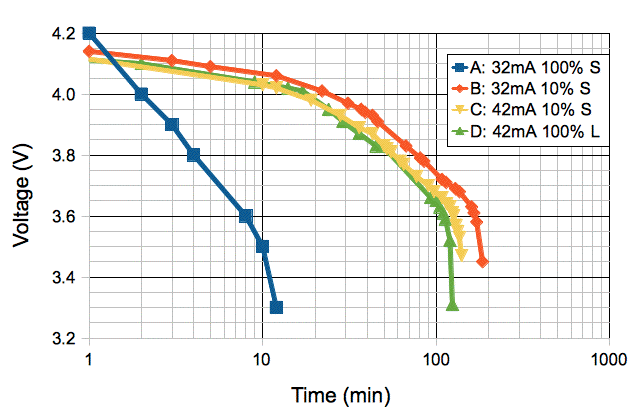
Figure: Discharge of Lithium-Ion Batteries for Various Currents. Plots A, B, and C are for the small (S) 19 mA-hr battery. Plot D is for the large (L) 150-mHhr battery. We specify the duty cycle of the discharge current in each case.
A: The battery is , charged up two months ago. We run 32 mA through the lamp continuously. The battery current is 50 mA for VBAT = 3.6 V. The battery runs for 12 minutes, delivering roughly 10 mA-hr.
B: We re-charge the same battery. We run 32 mA through the lamp for 1 ms out of very 10 ms. The battery current is 6.7 mA for VBAT = 3.6 V. The battery runs for 190 minutes, delivering roughly 21 mA-hr.
C: We re-charge the same battery. We run 42 mA through the lamp for 1 ms out of every 10 ms. The battery current is 8.4 mA for VBAT = 3.6 V. The battery runs for 140 minutes, delivering roughly 20 mA-hr.
[12-FEB-14] We equip A3024B No2.1 with a 382030 lithium-ion battery, capacity 160 mA-hr, maximum recommended discharge current 160 mA. This particular battery is one we have charged and discharged many times at various rates. We charge it up and solder its leads to the A3024B circuit board. We connect A3024HFB No2.2 through 100 mm stretched springs with resistance 52 Ω. We turn on the LED. Forward voltage drop is 2.88 V, lamp voltage from boost regulator is 5.09 V. Lamp current must be 42 mA. Graph D above shows discharge of this battery with continuous 42 mA to the lamp, which is 65 mA from the battery. The battery runs for 125 minutes, delivering roughly 140 mA-hr.
Encapsulation
[21-AUG-14] We encapsulated our A3024B-M and A3024B-R with clear, five-minute epoxy and then four coats of silicone. The silicone is about 1 mm thick all around. The epoxy coats the circuit and battery, making a better surface for the silicone to adhere to. We did not apply an acrylic coating to the circuit board, nor did we place the epoxy in a vacuum to remove cavities. There would have been little point in trying to remove cavities when the setting time of the epoxy was only a few minutes.
When Rob Wykes implanted the head fixture, he was concerned about its height, which reached over 10 mm, but he covered it with dental cement, anchored it with three skull screws, and after nine weeks of implantation, both head fixtures were still secure, and both rats were healthy. The implantable lamps performed well after five weeks of implantation, but after nine weeks, No2.6 did not respond at all, and No2.1 responded only when the antenna was adjacent to the animal.
The lamp circuits were removed in July and shipped back to us in August. The photograph below shows corrosion on pins and pads carrying VBAT.

Figure: Corrosion of Pins and Pads Carrying VBAT After Nine Weeks Implanted, A3024B-R No2.6. Click for higher resolution.
The battery voltage in the above circuit remains 3.4 V, but we cannot get lamp power out of the leads. The part on the left is U2, the boost regulator, and the part on the right is U1, the comparator. We see no trace of metal left in U2-6 or U1-5, the power supply pins for the two components. Meanwhile, circuit No2.1 now responds perfectly, with good operating range. But it, too, shows corrosion in the same location.

Figure: Corrosion of Pins and Pads Carrying VBAT After Nine Weeks Implanted, A3024B-R No2.1. Click for higher resolution.
In No2.1 we do see metal left in U2-6 and U1-5. Condensation across R1, a 10-MΩ resistor, would cause the device's power threshold to rise. The corrosion is a certain signe of condensation within the encapsulation, so we suspect that the poor responsivity of No2.1 was due to a drop in the effective value of R1.
We hope to solve these encapsulation problems with an acrylic coating in future Implantable Lamps.
Fiber Construction
You will find instructions for making tapered glass fibers here.
Conclusion
[21-FEB-14] We have five head fixtures and five implantable lamps ready to ship to ION. Shown below are 3 of A3024B-M (mouse-sized) and 2 of A3024B-R (rat-sized) implantable lamp with lithium-ion battery. Each circuit is encapsulated in clear epoxy and four coats of silicone. Each lead is terminated with a 300-μm diameter gold-plated pin. The red lead is L+ and the blue is L−.

Figure: ISL Stage Four Delivery of Implantable Lamp Circuits, A3024B-M and A3024B-R. The blue line is 50 mm long.
The operating range of these lamps for command reception in our basement office is at least three meters. But one of our concerns with the mouse-sized A3024B-M is the size of the antenna, combined with the short length of the leads. We are not sure how the surgeon can implant this device in a mouse with the antenna maintaining its shape and the leads reaching the skull. If the surgeon finds that there is insufficient space to accommodate the antenna as it is, he should feel free to deform its shape. Deformation of the antenna will reduce operating range for command reception, but we expect the range will still be over 100 cm.
The table below lists the characteristics of each lamp. We estimate the transmitter volume from caliper measurements. We charged the batteries just before encapsulation. We measure the lead resistance with a meter. The current delivered by a lamp circuit is limited by the resistance of its leads. Lamp circuit No2.4 has two solder joints in its leads at the base, where we replaced unstretched leads with stretched leads to allow the circuit to deliver more current.
| Circuit
Number | Battery
Capacity | Body
Volume | Lead
Length | Lead
Type | Lead
Resistance |
| 2.1 | 160 mAhr | 4.8 ml | 100 mm | Stretched | 56 Ω |
| 2.2 | 19 mAhr | 1.7 ml | 50 mm | Unstretched | 55 Ω |
| 2.3 | 19 mAhr | 1.7 ml | 50 mm | Unstretched | 55 Ω |
| 2.4 | 19 mAhr | 1.7 ml | 50 mm | Stretched | 29 Ω |
| 2.6 | 160 mAhr | 4.8 ml | 100 mm | Stretched | 56 Ω |
Table: Characteristics of ISL Stage Four Implantable Lamp Circuits.
The photograph below shows one of five A3024HFB head fixtures. There is some deliberate variation in the way we aligned the fiber tip and the guide cannula. Click on the head fixture names to get a close-up picture of each one. In all cases, the fiber's outer diameter is close to 450 μm. The head fixture shown below is No2.11, an A3024HFB-G green lamp. Note that the glue does not extend to the contact between the guide cannula and the taper. In some head fixtures, the contact point is glued, in others it is not. In the former, we are sure there is no glue on the taper. In the later, we know that the guide cannula is fragile. We are also shipping A3024HFB-B No2.4, 2.9, 2.6, and A3024HFB-G No2.12. All are equipped with two sockets that accept 300-μ diameter pins. the L+ connection is marked "+" on the circuit board, and the L− connection is marked "−".

Figure: ISL Stage Four Head Fixture A3024HFB-G. This one is shown without its dummy cannula. We ship all head fixtures with a dummy cannula threaded onto the guide cannula.
The characteristics of each head fixture are given in two tables for the blue and green versions. Any implantable lamp may be combined with any head fixture. By choosing which lamp circuit to combine with which head fixture, we can obtain more or less power at the fiber tip, and more or less operating life. The following table shows some example combinations.
| Circuit
Number | Battery
Capacity | Lamp
Number | Light
Power | Light
Color | Lamp
Current | 100% Duty
Life | 10% Duty
Life |
|---|
| 2.4 | 19 mAhr | 2.4 | 22 mW | Blue | 70 mA | 5 min | 2 hrs |
| 2.6 | 160 mAhr | 2.12 | 6 mW | Green | 40 mA | 2 hr | 20 hrs |
| 2.2 | 19 mAhr | 2.9 | 13 mW | Blue | 42 mA | 10 min | 3 hrs |
Table: Light Output and Operating Life of Various Combinations of Lamp Circuits and Head Fixtures.
If the capacity of a lithium-ion battery is C mA-hr, it can deliver up to C mA continuously while delivering its full capacity. At higher currents, its capacity decreases. But if it is allowed to recover after short bursts of higher current, it can deliver close to its full capacity. We present discharge graphs for our lamp circuit batteries here.
According to Bernstein et al., "To activate channelrhodopsin-2 and halorhodopsin molecules in mammalian neurons requires light of the appropriate color at a radiant flux of 10 mW/mm2 or greater, for maximal activation. A radiant flux of 1 mW/mm2 will activate approximately 50% of the molecules, and a radiant flux of 0.1 mW/mm2 will activate very few of the molecules." Light power density will drop with range from our fiber tip due to the geometric inverse square law, scattering, and absorption. Scattering causes power loss only because it encourages absorption by increasing the effective path length from the fiber tip. According to Johansson, the absorption coefficient of brain tissue is 0.35 mm−1 at 460 nm and 0.25 mm−1 at 527 nm. The scattering coefficient is around 1.2 mm−1 for both wavelengths.
Along a 1-mm path in the brain, 70% of photons will be scattered. Most of them will travel around 1.5 mm to arrive 1 mm from their starting point. Along this 1.5 mm path, 40% of 460-nm photons and 30% of 527-nm photons will be absorbed. If we consider a hemisphere around the base of our fiber tip, of radius 1 mm, its area is 2π mm2. If the fiber tip emits 13 mW of 460-nm light, the intensity on the surface of this hemisphere will be of order 13 mW / 2π mm2 × 60% = 1.2 mW/mm2. For 6 mW of green light we get 0.67 mW/mm2 at the same range. Our calculation is optimistic in that we assume the light is confined only to a hemisphere, but pessimistic because it ignores the fact that the light is being emitted all along the fibre tip, so the path length of most photons to the hemisphere surface will be shorter than we have assumed.
Thus we believe our head fixtures deliver over 1 mW/mm2 of 460 nm light and over 0.5 mW/mm2 of 527 nm light at a range of 1 mm from the fiber tip, which should be sufficient to excite over 50% of opsin molecules in a 1-mm diameter hemisphere around the fiber.
[21-AUG-14] This past June, two A3024B-R implantable lamps produced optogenetic behavior rats five weeks after injection of an opsin. We describe the experiments in more detail in Optogenetic Behavior Observed. Both the lamp circuit and the head fixture performed well and fulfilled their function as prototypes for the Implantable Sensor with Lamp. We did not apply an acrylic coating to the circuit before encapsulating, and after nine weeks of implantation, both circuits show severe corrosion of pins and pads due to condensation while implanted (see No2.1 and No2.6). Our hope is that an acrylic coating will stop such corrosion in the same way that it does so for our subcutaneous transmitters. For the next version of the implantable lamp circuit, see the Implantable Sensor with Lamp (A3030A).
Appendix: Batch ISL4C
[15-SEP-14] We have a batch of 8 of A3024HFC-B. The power sockets on the C version are on the same side of the circuit board as the LED, so the pins will be inserted from the bottom side during implantation. The guide cannulas are cut 9 or 10 mm below the pedestal. Those with the 10-mm cut proide 1 mm more space between the pedestal and the circuit board for glue, as shown below.

Figure: ISL Stage Four Head Fixture A3024HFC-B. This circuit has not yet been clipped from the connector extension.
The guide cannula is made of silica, and so is fragile in the 2-mm span between the pedestal and the circuit board. Head fixtures 2.7, 3.1-3.5 all have the 10-mm cut, while No2.2 and 2.5 have the 9-mm cut. All eight head fixtures are intended for use with 5-V drive and 50-Ω leads. Given the forward voltage drop of around 3.0 V, we expect a drive current of 40 mA. The table below gives the LED power output and the power we measured at the tip for a 40-mA drive current.
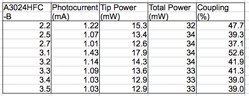
Figure: Output Power and Coupling Efficiency of A3024HFC-Bs. The output power is for 40 mA forward current.
Head fixture No2.2 we previously found to have 22% coupling efficiency, but repeated measurements over the past two months show coupling of around 45%, and today we measure tip power 15 mW at 40 mA forward current. This head fixture is unusual in that we placed the fiber base off-center by 200 μm.
Head fixture No3.1 provides 18 mW at the tip for 40 mA forward current, and coupling efficiency 53%, which matches our theoretical maximum for a 450-μm fiber with numerical aperture 0.86. This head fixture is unusual in that we soldered the LED package poorly, so it was inclined at an angle of 3.5° to the circuit board. Instead of re-soldering the package, we went ahead and lowered the fiber base into position, just to see what would happen. The figure below shows the inclined package. Because of the incline, we could not place the fiber directly on the LED.
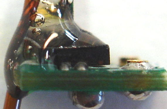
Figure: ISL Stage Four Head Fixture A3024HFC-B. This head fixture is remarkable for its apparent 53% coupling efficiency, but it could be that the light emission is asymmetric, and we measured on the bright side.
For shipment to ION we select No2.2, 2.5, 3.1, 3.2, and 3.3. These include three with the 10-mm guide and two with the older 9-mm guide.
Appendix: Batch ISL5
[14-NOV-14] We present the five A3024HFC-B head fixtures for ISL Stage 5 are photographed in ISL Stage 5 Delivery. Taper tip power is 13-15 mW at 40 mA LED current.
Appendix: Batch ISL6
[23-APR-15] We measure the lead resistance of each lamp lead of our C6.1-7 A3030C ISLs and get 31±1 Ω. The forward voltage of our C460EZ500s is 2.9 V at 40 mA. The lamp power output voltage of the A3030C is nominally 5.1 V. Our lamp current will be approximately 34 mA. Average taper power output of our latest fixtures is 14.5 mW at 40 mW forward current, so we expect the power output when implanted to be 12.3 mW.
[04-MAY-15] We have A3024HFC-B No6.1-8 and No2.7 for ISL6. The No6.4 failed by shorted bond wire. The remainder have light output 13-16 mW at 40 mA. The No6.8 LED was inclined by a few degrees.
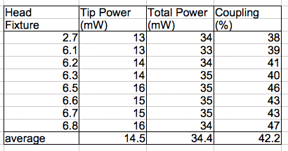
Figure: Output Power and Coupling Efficiency of ISL6 Head Fixtures at 40 mA LED Current.
The remarkable No3.1, which appeared to emit 18 mW, and which included an angle of 3.5° between the photodiode and the fiber base, may have been brighter on one side because of this angle. The angle might biase emission of light in the sideways directions rather than the forward. Our photodiode method would give us a higher estimate of total output power. We measured power output on all four sides of No6.8, which also had an angled LED, and provides 16 mW output power. All sides were the same. We measured forward power with our 10-mm square photodiode and obtained 10.2 mW. With No6.1 emits 9.1 mW in the forward direction, and our estimate of total power was 13 mW. We see no evidence of distortion of the emission field due to the angle at the base.
We equip the ISL6 head fixtures with 10-mm long silica cannula guides.
Appendix: Batch ISL7
[22-JUN-15] In ISL5 and ISL6, we made no use of the guide canula during the implantation, nor afterwards. For ISL7, we attach the guide cannula in such a way that it may be used to hold the head fixture in place during implantation, but later be cut off.

Figure: Head Fixture for ISL7 (A3024HFD-B).
[04-JUL-15] ION prefers the A3024HFC for ISL7. We have ten head fixtures out of fifteen completed so far.

Figure: Silica Guide Cannulas.
We run out of silica cannula guides and have no time to wait for more, so we use 10-mm steel cannula guides instead.

Figure: Steel Guide Cannulas.
[16-JUL-15] This photograph shows the fifteen head fixtures of Batch ISL7. The following table lists the head fixtures, their configuration with guide cannula and LED, and their performance.

Figure: Output Power, Color, and Cannula Type for ISL7 Head Fixtures. We measure optical power with a photodiode and 40 mA LED current. All head fixtures are A3024HFC, except 7.1, which is A3024HFD.
The minimum diameter of the fibers we used to make these head fixtures was 440 μm, but we had some that were 460 μm. According to our calculations, the theoretical maximum coupling efficiencies for these diameters and our higher-index fiber is 48-52%. We see that we achieve the theoretical maximum in one head fixture.
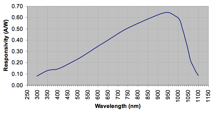