Data Transmission and Reception Circuits, Part Two
© 2006, Kevan Hashemi Open Source Instruments Inc.
Contents
Introduction
Interference Spectra
Operating Frequency
Modulation Spectra
Versatile Transmitter
Message Encoding
Demodulating Receiver
Data Recorder
Data Receiver
Software
Foreign Interference
Maximum Range
Power Transmission
Multi-Path Interference
Omnidirectional Antennas
Hand-Held Operation
Operating Range
Analog Inputs
Peer-to-Peer Interference
Battery Life
Temperature
Assembly
Deliveries
Conclusion
Introduction
In our Technical Proposal, we layed out our plan to develop a transmitter small enough to be implanted in the body of a rat, fast enough to transmit four hundred data samples per second, powerful enough to be detected at a range of three meters, and efficient enough to operate for three months on a lithium battery. We divided our development into four stages.
- Technical Proposal (£3000)
- Dummy Transmission Circuits (£5000)
- Data Transmission and Reception Circuits (£5000)
- Prototype Circuits (£7000)
Stages One and Two we completed with success. Our first attempt to complete Stage Three was a failure. Our data transmission and reception circuits worked well in our basement laboratory in the United States, but did not work at all in the Institute of Neurology's (ION) tenth-floor laboratory in London.
In Part One of this report, we described how interference from cell phones was to blame for the failure at ION, and concluded that a better choice of operating frequency, and a few improvements to the transmitter's method of modulation, would suffice to overcome the interference.
Here we show how the new Subcutaneous Transmitter (A3009) and Demodulating Receiver (A3005C) overcome interference to give robust, short-range communication. We describe how the Data Recorder (A3007) picks out A3009 transmissions from noise and interference, and stores them in its own memory. But we begin with measurements of interference power spectra obtained with our new RF Spectrometer (A3008) in both Boston and London.
Interference Spectra
After the failure of our transmitters in London, we concluded that we needed an instrument that could measure radio-frequency power density in the range of frequencies accessible by our transmitters. That is so say: we needed a radio-frequency spectrometer. We found nothing for less than $5000 available commercially, and we knew we would need to send one to London, and have another for ourselves, so we designed and built our own. The RF Spectrometer (A3008) measures relative RF power in 3-MHz wide bands in the range 875 MHz to 1050 MHz.
In this and the following sections, we present many spectra obtained with our Spectrometer tool. We provide you with links to the raw data, in case you want to load it into the Spectrometer tool yourself and take a look at it, or plot it for yourself. The raw data are text files saved from the Spectrometer instrument with the Save button. Each line in a file gives a graph letter, a spectrometer frequency index, and the measured power. The plots you see all draw a blue line along the bottom at +20 dB. So a value of +30 dB in the raw data appears in a plot at +10 dB above the blue line.
Matthew Walker obtained the following spectra in London.
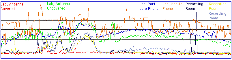
Figure: RF Power Spectra in the Institute of Neurology, London. The vertical lines mark 20-MHz bands, starting with 880 MHz on the left edge of the graph. The horizontal lines mark relative power density in +10 dB increments. One division higher means ten times the power density.
Whenever we take a collection of spectra, we always cover the antenna at some point, to measure the spectrometer's inherent noise, and we expect this distribution to be flat with frequency. Even with the antenna covered, however, we still get some features in our spectrum. A foil cover can't keep out all external fields. But let's ignore these bumps, and draw a stright line along the covered-antenna spectrum, to obtain the background noise power. We define dBn as a measure of power with respect to the background noise. The power of a signal in dBn is the number of decibels by which its power exceeds that of the thermal background. If a new spectrum is 10 dB above the covered-antenna spectrum, we say it's power density is +10 dBn.
When we uncover the spectrometer antenna, but leave our own transmitters turned off, we measure the background interference power. We define dBi as a measure of power with respect to the background interference in our transmission band. If our transmitter spectrum is 10 dB above the average interference power in our transmission band, we say it's power density is +10 dBi.

Figure: RF Power Spectra at Brandeis University, Boston. The vertical lines mark 20-MHz bands, but the frequency at the left edge of the graph varies with temperature, as you can see from the location of certain common features. At 19 °C, the left side of the graph is 870 MHz, and the fifth line from the left is 950 MHz. The horizontal lines mark +10 dB increments in power density.
Our A3006 operated by transmitting in the 930-970 MHz band to send a one, and in the 880-920 MHz band to send a zero. We confirmed this with the spectrometer, as you can see here. The A3006 worked fine in Boston because we observed less than +3 dBn interference in the 930-970 MHz band. But in London, we observed over +20 dBn interference in the same band. Even when the A3006 was transmitting in the 880-920 MHz band, to indicate a zero, our receiver continued to receive power in the 930-970 MHz band, and therefore received ones.
On July 3rd 2006, we obtained the following spectra on a window sill in the Annex of Kevan's parents' house in Guildford, England.

Figure: RF Power Spectra in Guildford, UK. The vertical lines mark 928 and 960 MHz. Red (A): background interference. Green (B) ISM-band transmitter at 30 cm with ±12 MHz modulation. Blue (C) ISM-band transmitter at 30 cm with ± 8 MHz modulation. Raw data here.
(For further discussion of background interference, see here.)
Operating Frequency
After some investigation on the web, Matthew Walker determined that the 902-928 MHz band was available for unlicensed use in the United Kingdom, and we determined that the same was true in the United States. This band is called the 900 MHz ISM band, where ISM stands for "Industrial, Scientific, Medical".
Although there is up to +20 dBn interference in the ISM band in Matthew's office in London, this intereference drops to around +10 dBn in his animal laboratory. The power transmitted by an A3006 is as great as +30 dBn at range 60 cm. We anticipate that our signal power need exceed the interference power by only 6 dB for the interference to be dominated in our frequency-demodulating receiver.
Given that operation in the ISM band is possible both in Boston and London, and requires no consultation with regulatory organisations, Matthew Walker chose the ISM band for the second batch of Stage Three transmitters.
Our RF Spectrometer is a fine instrument, but its absolute frequency accuracy is only ±5 MHz from one spectrometer to the next, and ±2 MHz with ±10°C changes in temperature. The spectrometer does provide SAW filters with which to calibrate itself, but we find this self-calibration clumsy and time-consuming.
Our ultimate frequency reference for our ISM band operations will be the SAW filters in our Demodulating Receivers (A3005C). These are the B3588 from Epcos. They provide a 30-MHz pass-band as shown below.
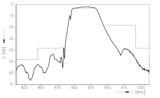
Figure: Frequency Response of B3588 SAW Filter.
Our A3005C's pass band extends from roughly 890 MHz to 930 MHz, which is a total of 40 MHz. The strict ISM band extends only from 902 MHz to 928 MHz, giving us only 25 MHz to work in.
(For our original discussion of a change to the ISM band, see here. For a more detailed discussion of frequency band allocation, see here.)
Modulation Spectra
As we describe here, our new transmitters will modulate their transmission frequency entirely within our chosen frequency band. In the ISM band, whose center lies at 915 MHz, we might transmit at 920 MHz for a one, and 910 MHz for a zero. The number of times we switch to and from each frequency per second is our modulation frequency. When our modulation frequency is much smaller than the separation of the two carrier frequencies, the power spectrum will consist of two peaks, one at the lower carrier frequency, and one at the higher. But as the modulation frequency becomes comparable to the separation in carrier frequencies, these peaks will spread out, interfere with one another, and create a more complicated spectrum. With some effort, we can calculate the resulting spectrum, and when we do so, we find that it is a combination of Bessel Functions. Alternatively, we can measure the spectra of a modulated carrier frequency with our RF Spectrometer (A3008).
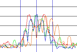
Figure: Spectra of Modulated Carrier. The three vertical blue lines mark 902 MHz, 915 MHz, and 928 MHz, calibrated with respect to a A3005C ISM-band SAW filter. In each case, the transmitter switches between a lower frequency, f0, and a higher frequency, f1, with modulation frequency fm. Red: f0 = 910 MHz, f1 = 920 MHz, fm = 500 kHz. Green: f0 = 910 MHz, f1 = 920 MHz, fm = 5 MHz. Blue: f0 = 910 MHz, f1 = 920 MHz, fm = 5 MHz sin wave instead of square wave. Orange: f0 = 915 MHz, f1 = 925 MHz, fm = 5 MHz.
We performed the above measurements with the apparatus shown here. The transmitter is our trusty old Modulating Transmitter (A3001A). In addition to the RF Spectrometer, we also record the output from a Demodulating Receiver (A3005C), as we will show you below. As you can see in the photograph of the apparatus, the Modulating Transmitter is roughly 70 cm from the RF Spectrometer. The RF Spectrometer receives +30 dBi from the Modulating Transmitter at the center of the transmission spectrum.
The Modulating Transmitter uses the same MAX2624 chip to generate its RF power as our Subcutaneous Transmitters. Our measurements suggests that the Modulating Transmitter output power is approximately equal to that of the Subcutaneous Transmitter (after we install the decoupling capacitor C11). We expect the transmission spectrum from a Subcutaneous Transmitter in the same orientation at range 70 cm to be roughly the same, at +30 dBi.
The green trace we obtained with a 5-MHz square wave driving the Modulating Transmitter input, while the blue trace we obtained with a 5-MHz sine wave. The spectrum changes hardly at all between the two, which tells us that the Modulating Transmitter is insensitive to the higher-order harmonics in the square wave. This and other observations lead us to conclude that the modulation bandwidth of the MAX2624 is roughly 5 MHz.
The blue lines in the above graph mark the edges of the ISM band. Power outside these blue lines will not pass through the ISM-band SAW filter in the A3005C's antenna amplifier. The green trace fits into the ISM band with roughly 2.5 MHz to spare on either side. Of course, there is some power in the spectrum outside the ISM band, but we get 95% of the power within a 20-MHz band centered at 915 MHz, and therefore extending from 905 MHz to 925 MHz. The ISM band extends from 902 MHz to 928 MHz.
When we shift our carrier frequencies up by 5 MHz, we get the orange trace. Although the carrier frequencies lie within the ISM band (they are at 915 MHz and 920 MHz), 20% extends above 928 MHz (to the right of the right-most blue line).
Versatile Transmitter
The Subcutaneous Transmitter (A3009) drives its radio-frequency (RF) voltage-controlled oscillator (VCO) with a five-bit digital-to-analog converter (5-bit DAC). The 5-bit DAC consists of five resistors, R4 to R8 in the schematic, connected to 1.8-V logic outputs at one end and the VCO input at the other end. The DAC allows the A3009 to set the TUNE input in steps of 1.8 V / 32 = 56 mV. The VCO tuning curve shows an approximate slope of +70 MHz/V, so the DAC can control the output frequency in steps of 4 MHz.
We can program the A3009 to transmit in any frequency band between 880 MHz and 1000 MHz. We describe how to calibrate and program an A3009 to transmit in the ISM band here. The rate at which it transmits messages is also programmable. The frequency response of its three-pole low-pass filter, and its one-pole high-pass filter we can change by choosing different capacitor values.
It was not until 22-JUN-06 that we discovered that the addition of C11 in the schematic increases the RF power transmitted by the A3009 by a factor of four (+6 dB). The existing power supply decoupling for the MAX2624 oscillator was inadequate. Since then, we have added C11 to all transmitters.
Message Encoding
The A3009 message encoding is more complicated than that used by the A3006. To transmit a one-bit, we don't simply transmit at our one-frequency. Instead, we transmit at our zero-frequency for 100 ns, and then at our one-frequency for 100 ns. To transmit a zero-bit, we transmit at our one-frequency for 100 ns, and then at our zero-frequency for 100 ns. Here's an example A3009R transmission.

Figure: A3005C Output for A3009R Transmission. The A3009R is transmitting at 911±8 MHz. The top trace is the A3005C output. The bottom trace is the frequency-value output from the A3009R.
The A3009 provides a frequency-value logic output, which you can get to when it's plugged into an SCT Programmer (A3011). For a photograph of the apparatus we used to obtain the above traces, see here, and for more discussion of calibrating an A3009, see here. When the frequency-value HI, the A3009 is driving its VCO to its one-frequency.
The A3009 begins its transmission by turning on its VCO and transmitting a string of ten one-bits. By the fifth or sixth one-bit, the Data Recorder (A3007B) watches the rising edges of the incoming signal. It knows when to expect the next rising edge, because it has received the previous one, and it knows that the rising edges will be separated by approximately 200 ns.
After ten one-bits, the A3009 transmits a zero-bit. The Data Recorder has been watching for a rising edge, but instead is sees a falling edge. It knows now that the data part of the tranmission has begun, and it watches for the next data edge 200 ns later. It ignores the set-up edge that may or may not occur 100 ns after the data edge.
In this way, the Data Recorder moves from one data edge to the next, always skipping over the set-up edges. The match between the Data Recoder's clock and the A3009's clock need not be precise. So long as they each agree about what 100 ns is to within 20%, the communication will work. Because of this loosening in the timing constraints, the A3009 ring oscillator frequency can vary by up to 20% without affecting communication.
But the greatest benefit to our using edges to transmit data is that the message itself can be high-pass filtered and low-pass filtered before translation into logic levels. The simple resistor-capacitor circuit at the Data Recorder (A3007B) input does both, as you can see in the schematic. The high-pass filter means that we eliminate the DC offset in the A3005C's output. We can shift the center frequency of our transmitter, which changes the DC offset of the A3005's output, without affecting the high-pass filtered signal. Because of this, all the Demodulating Receiver (A3005C) has to do is provide a positive derivative in its output with respect to frequency, while the Subcutaneous Transmitter (A3009) has only to modulate between two frequencies within the ISM band.
For example, one A3009 might transmit at 911±4 MHz, while another transmits at 919±4 MHz. The output of the A3005C will look the same for both, except the second signal will be raised by roughly 50 mV compared to its amplitude of 100 mV. This substantial DC offset disappears when the signal passes through C4 in the Data Recorder (A3007B).
Our use of edges to transmit logic bits increases the bandwidth of our transmitted signal, but makes reception and transmission more robust. In particular, there is so much timing information in the encoded signal that the Data Recorder (A3007B) can pick out A3009 messages from the random sequence of transitions produced by thermal noise and interference in the Data Receiver (A3005C) output.
You can see how the A3009 performs its encoding by looking at its logic chip firmware. Unless you understand the ABLE programming language, however, the firmware code won't mean that much to you. You could also examine the receiver section of the A3007 firmware, but it's even more complicated and lengthy than the A3009 firmware.
The A3009 transmits four ID bits, which represent an identifying number between 1 and 14. The number 0 is reserved for the Data Recoder's time stamps, and the number 15 is reserved for future use. After the four ID bits comes sixteen ADC bits. In the case of a reference transmitter, A3009R, these bits are generated by the logic chip itself, and represent a square wave, or some other regular waveform. After the sixteen data bits come the four ID bits again, but this time they are inverted, althogh they are in the same order.
Demodulating Receiver
The A3005C is a modified version of the A3005A. It's RF band-pass filter covers the ISM band. It has more gain, so that thermal noise causes its amplifier to saturate, and we always see a demodulated output. The A3005C offsets its local oscillator frequency to produce a positive derivative in its output with respect to frequency. We describe the evolution of the A3005C out of the A3005A here.
The A3005C requires adjustment of its LO frequency to set its response correctly for demodulation. We do this by connecting our Modulating Transmitter to a triangle wave, and sweeping its frequency through the ISM band.

Figure: Apparatus for Adjusting A3005C, and Testing Modulation Bandwidth. The Demodulating Recevier (A3005C) is on the lower-right, with an RF Spectrometer (A3008) just to the left of it. On the opposite side of the tableis our Modulating Transmitter (A3001). The oscilloscope sits on top of our function generator.
We adjust VR1 in the A3005C Local Oscillator circuit until we see something like the following on the oscilloscope.
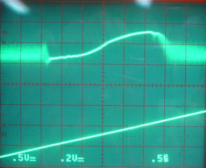
Figure: Frequency Response of Demodulating Receiver A3005B. The top trace is the A3005C output. The bottom trace is the TUNE input of the VCO on our Modulating Transmitter. Zero volts is the very bottom line in the red scale. The A3005B differs from the A300C only in that it uses a 947±13 MHz SAW filter instead of the A3005C's 915±13 MHz filter.
The trace shows amplified and demodulated thermal noise on either side of a positive noise-free gradient. The noise-free output occurs when the Modulating Transmitter output sweeps through the pass-band of the A3005C's SAW filter. The noise occurs elsewhere. The SAW filter rejects the Modulating Transmitter output, leaving interference and thermal noise to driver the A3005C output.
We adjust VR1 until we get a positive slope with respect to frequency as shown in the figure. We must be sure to let the A3005C reach its equillibrium temperature before we make this adjustment, because the LO frequency drops as the MAX2624 warms up, and this moves the response peak to the left.
Having adjusted the LO frequency, we can test the modulation bandwidth of the MAX2624 on the Modulating Transmitter, in combination with the amplifiers and filters on the A3005C. We begin with a 500-kHz square wave driving the transmitter between approximately 910 MHz and 920 MHz. We see a clean square wave in the response. We increase the modulation frequency to 5 MHz, which matches that of the Subcutaneous Transmitter (A3009). Now we see a smoothed square wave in the response. As you can see, 5 MHz is pushing the limits of the modulation. Above 5 MHz, the response aplitude decreases. Our modulation bandwidth is close to 5 MHz. We show the spectra for these three measurements above.
Now we shift the transmission frequencies to 915 MHz and 920 MHz. This is the orange trace above. The transmission spectrum spreads outside the ISM band, and outside the nominal upper edge of our SAW filter's pass band. What happens to the A3005C response when we lose the upper lobe of the transmission spectrum? The response is asymmetric. Rising edges are slow, while falling edges are as fast as they were before. The rising edges are slowed down because the rising edges correspond to a move to a higher frequency, and the spectrum spread out to higher frequencies when this move occurs. Because the SAW filter is rejecting some of these higher frequencies, the rising edge is distorted. We conclude that if we want our response to remain fast in both directions, and therefore preserve our 5 MHz modulation bandwidth, we must make sure that 90% of the transmitted power lies within the pass-band of our SAW filter, which is typically 890 MHz to 930 MHz.
Data Recorder
The A3007B is a modified version of the A3007A, adapted for the new message encoding. It provides high-pass and low-pass filters on its input. It requires no adjustment.
Because the A3005C produces a constant demodulated output signal from thermal noise and interference, the Recorder's job is to pick out legitimate A3009 transmissions from what we assume to be a random series of logic transitions. These logic transmissions may be random, but they are bandwidth limited by the Recorder input filters to no more than 20 MBits/s. With this 20 MBit/s random sequence entering its Receiver state machine, we find that the Data Receiver (A3005C) produces a false messsage only once every half a second.
The A3007B checks each incoming message for timing errors that mark it out as noise, or distortion of the true and inverted ID bits that identify interference with an actual message. It will not accept a message with ID zero. Any message it accepts, it stores in its memory as three bytes (four ID bits, sixteen data bits, the inverted four ID bits) and a one-byte time stamp. The total message record is four bytes long.
Every 256 periods of its 32.768 kHz reference oscillator, which is every 7.8 ms, the A3007B records a time stamp message in its memory. The time stamp takes the form of a message from a transmitter with ID zero, and its sixteen bits of data are the value of a sixteen-bit timestamp counter.
The A3007B has a 24-bit counter running off its 32.768 kHz oscillator. Every time the lowest seven bits of the counter are zero, it records a time stamp message containing the top sixteen bits of the counter. The time stamp byte at the end of each message is the bottom eight bits of the counter. The bottom eight bits of each time stamp message are always zero, but the time stamp bits at the end of the other messages, in combination with the time stamp messages, allow us to determine exactly when they occured within a 512-second window. We leave it to the data acquisition computer to settle where this 512-second window lies in comparison to real time.
The A3007 stores its data in a 512-kByte RAM buffer, waiting for block read-out by the LWDAQ Driver (A2037E). The first message stored is the first message to be retrieved, provided that the RAM buffer does not overflow. If it overflows, the old messages will be thrown away in favor of the new ones.
Each message occupies 4 bytes in memory. Each A3009 sends 512 messages per second, which occupies 2 KBytes of RAM per second. The A3007's time stamps get stored 128 times a second, which uses up 512 Bytes per second. If we have 10 A3009s operating simultaneously with one A3007, we are using 20.5 KBytes per second. The LWDAQ Driver can transfer A3007 data into its own RAM even while the A3007 is recording messages, and it can do so at over 1 MBytes/s. The A2037E driver can transfer only 160 KBytes/s over its Ethernet connection. Assuming the network to which the A2037E is connected can carry a steady 20.5 KBytes/s, we see that ten transmitters do not tax the data acquisition system.
Data Receiver
We combine the Demodulating Receiver (A3005C) and Data Recorder (A3007B) into a single box, which we call the Data Receiver (A3010), shown below with two A3009R transmitters. Users of the A3010 must be sure to let the box warm up for five minutes before expecting it to perform at its best. It takes about five minutes for the local oscillator chip inside to reach thermal equillibrium, at which point the A3005C has the best frequency response for operation in the ISM band.

Figure: Data Receiver (A3010A), showing enclosure, antenna, cable, and two transmitters.
For those of you interested in a peek inside the A3010A, see here.
Software
Starting with LWDAQ 6.0, the Recorder instrument operates only with the A3007B. You can see the red time-stamp trace plotted as if there were an additional transmitter with ID zero, transmitting the top sixteen bits of a twenty-four bit counter clocked by a 32.768 kHz oscillator.
The Stage Three software provides a display for testing the quality of reception from Subcutaneous Transmitters, but does not provide ways to record the incoming data to disk, or transfer it over the Internet to another computer. These improvements we leave to Stage Four of the development. We expect no technical challanges in making these improvements.Foreign Interference
Note: The A3009R we used in the following experiment did not have C11, the 100-pF decoupling capacitor across the MAX2624, as shown here. The transmitter output power started off 6 dB (four times) lower than it should have been.
Foreign interference was what defeated the Subcutaneous Transmitter (A3006) in London this February. Let's see how the Subcutaneous Transmitter (A3009) performs in the presence of interference. It's not so much the transmitter itself we need to test, but the transmission method: that of transmitting at two different frequencies within the receiver pass band to express two different symbols.
To begin with, we programmed an A3009R to transmit only at 915 MHz during its 8-μs transmission burst. This we did by centering its output frequency within the pass band of a Demodulating Receiver (A3005C), and setting its frequency_range to zero. To compete with the A3009R, we set up our Modulating Transmitter (A3001A) to switch between 920 MHz and 910 MHz at a rate slow enough that the frequency would almost always be constant during the A3009R's transmission burst, but fast enough that the result of both frequencies interfering with the A3009R's transmission would be visible on the oscilloscope screen at one time.
We arranged the A3001A, A3009R, A3005C, the function generator, and our oscilloscope as shown here, and varied the range of the two transmitter from the receiver. The figure below shows what we saw on the oscilloscope for various ratios of A3009R range to A3001A range.
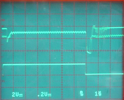

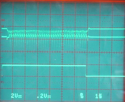
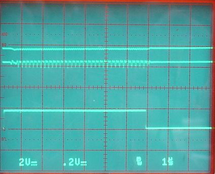
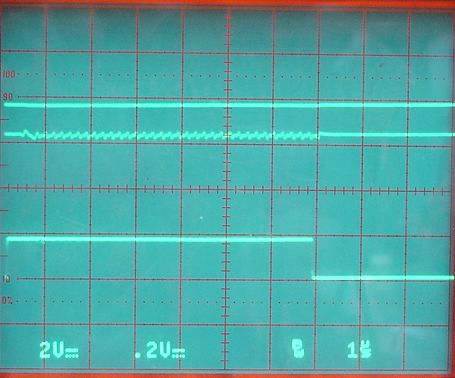
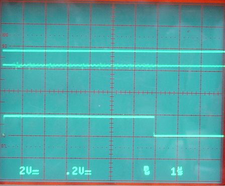
Figure: Competition Between A3009R and A3001A. Each oscilloscope display corresponds to different ranges of each transmitter from the receiver. The horizontal scale is 1 μs per division. From the top-left, proceeding as you would when reading, the ratio of the range of the A3009R to the range of the A3001A is 1:8, 1:4, 2:4, 4:4, 4:2, 4:1. In each case, one range unit is roughly 20 cm.
In the 1:8 result, we see the A3009R dominates the A3001A transmission almost completely. The straight line in the top trace, with slight ripples in it, indicates reception at 915 MHz. The A3001A dominates the A3009R almost completely when the range ratio is 4:2. The two straight lines with slight ripples in them indicate transmission alternately at 910 MHz and 920 MHz. For intermediate ratios, we see a gradual transition from the dominance of one transmitter to the dominance of the other.
Because the A3001A dominates the A3009R when it is at half the range, but the converse does not occur until the A3009R is at one eighth the range, we conclude that the A3001A emits a more powerful signal than the A3009R. Let us call the ratio of its ouput to that of the A3009R β, and we know that β>1.
The sensitivity of the A3005C across its 902-928 MHz operating range can vary by up to 3 dB because of ripples in the SAW filter pass band. But let us ignore these ripples, and assume them to be zero. In that case, dominance of one transmitter over another occurs when the power arriving at the antenna from the dominant transmitter is some fixed ratio higher than that arriving from the dominated transmitter. Let us call this ratio α. We previously predicted that when one sinusoid is three times more powerful than another, the zero-crossings of the sum occur with frequency nearly equal to the frequency of the more powerful sinusoid. Our receiver, with its high gain and limiting amplifiers, we designed to judge frequency on the basis of zero-crossings, in which case we hope to find that α ≈ 3.
At these close ranges, we can assume that reflected signals are much weaker than the line-of-sight signal. The power received from a transmitter is inversely proportional to the square of the range. When the A3009R is dominated by the A3001A at a range ratio of 4:2, the ratio of the power received from the A3001A to that received from the A3009R is:
(4/2)2β = 4β = α
When the A3009R dominates the A3001A at range ratio 8:1, the ratio of power received from the A3009R to that received by the A3001A is:
(8/1)2/β = 64/β = α
So we have 4β = 64/β, so β = 4 and α = 16. We were hoping to find α ≈ 3, so α ≈ 16 is a disappointment. To understand the discrepancy between our prediction and our observation, consider what would happen if we passed the receiver output through a low-pass filter with cut-off frequency around 1 MHz. Frequencies with period shorter than one horizontal division would be rejected by the low-pass filter. The ripples we see in the 1:4 image would be attenuated, leaving us with a straight line something like the 1:8 image. The two rippling lines in the 4:4 image would looke like the 4:2 image lines. With a 1-MHz low-pass filter, our observation of α would be:
(4/4)2β = β = α = (4/1)2/β = 16/β
From which we get α = 4 ≈ 3. We also get β = 4, as before, which makes sense: adding a 100-kHz low-pass filter to the receiver should not change the relative power output of the two transmitters. We see that α is a function of the bandwidth of the receiver output. The oscilloscope display is bandwidth-limited to 20 MHz (you will notice the little BW letter on the bottom of each image). With 20-MHz bandwidth, α = 16; with 1-MHz α = 4.
We now ask ourselves how we predict that we would need a 1-MHz low-pass filter to reduce α to 3. Consider the relative frequencies of the two interfering waveforms. In our prediction, we added sinusoids of frequency 1 Hz and 1.5 Hz. We can imagine measuring the frequency of the sum over ten cycles, which would be 10 seconds. Waiting for 10 s is similar to passing the demodulated output through a 0.1 Hz low-pass filter. Such a filter rejects any ripples at the difference of the two frequencies, which would be 0.5 Hz. In our observations, however, we're adding sinusoids of 915 MHz and 920 MHz. The difference between the two is 5 MHz. If you look closely at the 1:4 image, you can count the ripple cycles in one horizontal division. I count five, which is 5 MHz, the difference between the two interfering signals. If we want to acheive α = 3, we have to remove the difference frequency from our receiver output.
The A3009R transmission bandwidth is 5 MHz. The Data Recorder (A3007B) low-pass filters the receiver output at 10 MHz, using a single-pole RC network. This single-pole filter will attenuate 10 MHz ripples by 3 dB and 40 MHz ripples by 12 dB. Given that the difference between any two frequencies in the 902-928 MHz band is always less than 28 MHz, we see that this low-pass filter is of little use in rejecting the difference between an A3009R signal and a competitor in the ISM band. We cannot insert a sharp 1-MHz filter in the A3007B input, because we would reject our 5 MHz data. Because we are taking up the entire ISM band with our data transmission, we cannot reject interference with the theoretical minimum α ≈ 3. We must settle for α = 16.
In the light of these observations, we claim that our transmitter signal must be 16 times more powerful than interference and noise if it is to dominate and be received clearly. A factor of sixteen in power is 12 dB. We conclude that our transmitter signal must be at least +12 dBi to dominate the background interference.
Now let us consider the value of β we obtained. Both transmitters use the MAX2624 to generate their radio-frequency power. The A3001A has a dipole antenna with 50-Ω input. The A3009R has a quarter-wave antenna and a small ground plane. (For the more about antennas, see here.) The MAX2624 power supply is +5V in the A3001A and only +2.7 V in the A3009R. The dipole antenna may be more efficient than the quarter-wave antenna, and the higher supply voltage may increase the MAX2624 power output. Nevertheless, we doubted that these effect could reduce the transmitter efficiency by a factor of four.
We subequently discovered that adding a 100-pF decoupling capacitor across the MAX2624 on the transmitter increased the transmitter output power by 6 dB, as we show here. With C11 added, the A3009R dominates the A3001A when it is at one quarter the range (instead of one eighth), and the A3001A dominates the A3009R at one quarter range also (instead of one half). From this we conclude that β = 1.
Maximum Range
In the past, we measured the effect of antenna length upon transmitted power. We observed that if our antenna is half the optimal length, it radiates one quarter the power. If the radiated power is one quarter, we expect the range with the shorter antenna to be one half.
We arranged our Data Receiver (A3010) and our RF Spectrometer (A3008) on the floor as shown below. We attached a small wire to transmitter 2.4's battery, so make a tripod. You can see the transmitter standing up with a 40-mm bare antenna in the picture.
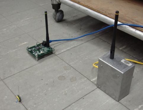
Figure: Apparatus for Measuring Power and Reception with Range.
The tiles on the floor are nine inches square. We moved the transmitter away one tile at a time until we were twenty-four tiles distant. At each step, we measured the peak power in dBi and noted whether or not our data receiver was getting a square wave from the transmitter. We performed the experiment for three antennas. The 80-mm insulated antenna is the thick red antenna shown here. The conductor is a stranded wire 0.5-mm in diameter. The red rubber insulation is 1-mm thick, making the total wire diameter 2.5 mm. The 80-mm bare antenna is the same piece of wire, but with the rubber insultation pulled off. The 40-mm bare antenna is the same piece of wire cut back to 40 mm.
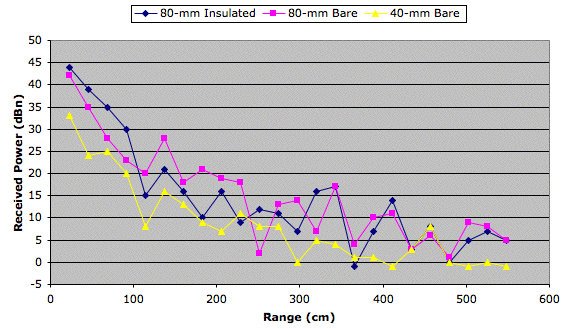
Figure: Received Power with Range. You will find the raw data as Range.xls in the zip archive here.
In the absence of reflections, the power received drops by 6 dB every time we double the range. We see such a decrease for the firste few tiles, but at range 1 m we begin to see the received power jumping up and down with range. These jumps are caused by reflections, as we described previously. Reflections are also called multi-path interference, which we discuss below.
We recall that we expect to get good reception when the received power is +12 dBi or higher. The graph below shows the state of reception at each range. When each graph is HI, we receive a square wave. When it is LO, we don't.
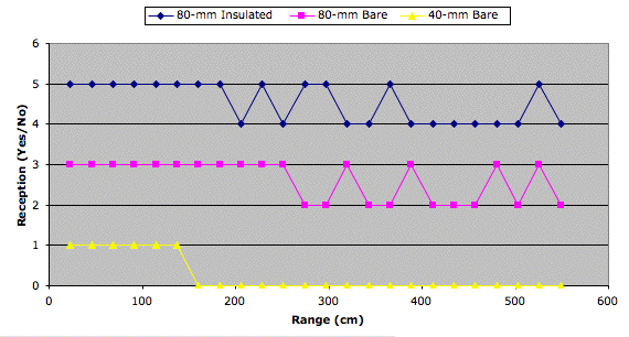
Figure: Reception with Range.
Because of reflections affecting the received power, the power received by the A3010 need not be the same as that received by the A3008. We cannot place the two antenna close together, or they will attenuate one another's received power. The relationship between reception and received power is therefore not clear from the above graphs. One graph corresponds to power received by the A3008, the other to power received by the A3010. But if we smooth out the jumps in the upper graphs, we see that reception does indeed start to fail at around +12 dBi.
We see no significant difference between the insulated and bare 80-mm antenna. The 40-mm antenna works up to 150 cm, while the 80-mm antennas work up to 250 cm. The 40-mm antenna appears to transmit one tenth the power of an 80-mm antenna at close range.
Power Transmission
In air, with an 80-mm antenna, our Subcutaneous Transmitter (A3009R) transmits as much power as our Modulating Transmitter (A3001A), provided we have added the decoupling capacitor C11, which we started doing on 22-JUN-06. At range 70 cm, the A3001A transmits +30 dBi to our RF Spectrometer (A3008). In the experiments below, we use the A3008 to measure the power transmitted towards the A3008R antenna, which is always vertical. We vary the antenna, its orientation, and the medium around the antenna. Our objective is to transmit power from inside a rat or a mouse. Their bodies are mostly water, so we try transmitting with water near the antenna, or with the entire transmitter immersed in water.
We placed an A3009R (number 2.4) 70 cm from our RF Spectrometer (A3008) and measured its power output for various types of antenna.
Figure: RF Spectra from A3009R with Various Antennas. The A3009R is at range 70 cm. Gray: 916-MHz commercial di-pole antenna on coaxial cable. Blue: 320-mm loop antenna connected to A3009R 0-V through 100-pF capacitor. Orange: 80-mm quarter-wave antenna. Black: helical antenna without cover. Yellow: helical antenna with cover.
For a photograph of the apparatus, see here. The photograph shows the loop antenna used to generate the blue trace. The dipole antenna was the ANT-916-CW-HWR from Antenna Factor. When combined with our A3009R output, ANT-916-CW-HWR transmits 3 dB less than either of our home-made antennas.
Figure: Helix Antenna With and Without Cover.
We extracted the helix from the ANT-916-CW-HWR, where it cooperated with a 70-mm tube to form a dipole. The helix is 4 mm in diameter, with 9 turns. If uncoiled, it is 130 mm long. For more about helical antennas, see below.
We attached transmitter 2.4 to a balloon full of air, in anticipation of subsequent experiments with a water-filled balloon. We measured the transmitter's power spectrum as seen by our RF Spectrometer (A3008) for various orientations of the balloon, at constant range 70 cm.
Figure: Air Balloon Supporting A3009R.
The transmitter's 80-mm quarter-wave antenna is held to the balloon with two rubber bands. The balloon and transmitter are in a pyrex dish, because we will be using a pyrex dish with our water balloons. The pyrex dish stops the water from a burst balloon from spilling all over our table. The following figure shows the orientations of the balloon we tried.
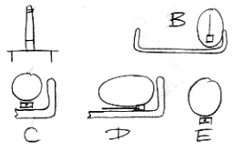
Figure: Orientations of the Air-Filled Balloon and Transmitter. The letters correspond to the graphs shown below. The top half of the drawing shows the pyrex dish, the spectrometer antenna, and the transmitter in orientation B. The smaller drawings below show the remaining orientations. The final drawing, E shows the pyrex dish removed.
For each orientation, we obtained an RF power spectrum, as shown below. You will find the raw data here. The red trace is the combined interference and noise power.
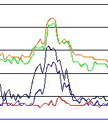
Figure: RF Spectra Obtained for Various Orientations in Air. Vertical divisions are 10 dB. The transmitter is 70 cm from the spectrometer. See the figure above for drawings of orientations. Red (A) transmitter turned off. Green (B) orientation B. Blue (C) orientation C. Orange (D) orientation D, Black (E) orientation E.
With the transmitter horizontal and tangential to the spectrometer antenna (orientations D and E), we see that the pyrex dish causes a 6-dB drop in received power. Either the pyrex is affecting resonance of the antenna, or it is absorbing the RF power.
Using our definition of dBi, the received power varies from +15 dBi to +35 dBi. We recall that the transmitter signal dominates when the received power is +12 dBi or more.
We replaced our air balloon with a water balloon. We strapped the same transmitter to the water balloon and placed the balloon in a pyrex dish, as shown below.
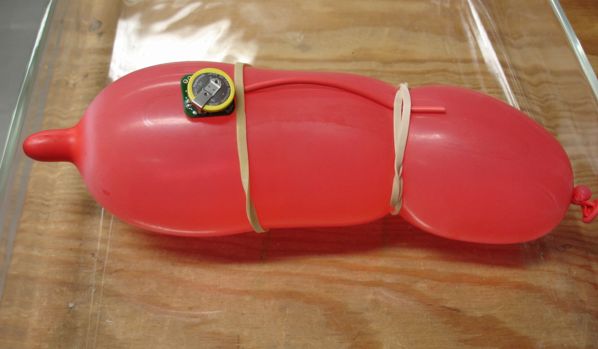
Figure: Water Balloon Supporting A3009R.
Once gain, we hold the 80-mm antenna to the balloon with rubber bands, and we hold the balloon in various orientations, as shown below.
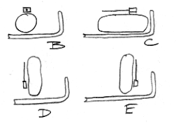
Figure: Orientations of the Water-Filled Balloon and Transmitter. The letters correspond to the graphs shown below.
In each orientation, we recorded the transmitter's radio-frequency power spectrum, as shown below. Graph A is the background spectrum. You will find the raw data here
Figure: RF Spectra Obtained for Various Orientations With Water Balloon. Vertical divisions are 10 dB. The transmitter is 70 cm from the spectrometer. See the figure above for drawings of orientations. Red (A) transmitter turned off. Green (B) orientation B. Blue (C) orientation C. Orange (D) orientation D, Black (E) orientation E.
The received power varies from +20 dBi to +23 dBi. Note, however, that we neglected to try the transmitter in orientation B, but with the transmitter beneath the balloon. It may be that the pyrex would, in that case, attenuate the signal by 5 dB, so that our minimum power would be +15 dBi with the water balloon. The minimum and peak power with an air balloon was +15 dBi and +35 dBi.
We cut back the antenna length from 80 mm to 10 mm in 10-mm steps, and measured the received spectrum from the transmitter strapped to the water balloon in orientation B. You will find the raw data here. We give the peak received power with antenna length in the table below.
| Antenna Length (mm) | Peak Power (dB) |
|---|
| 80 | 22 |
| 60 | 27 |
| 50 | 23 |
| 40 | 23 |
| 30 | 20 |
| 20 | 13 |
| 0 | 7 |
Table: Received Power for Various Antenna Lengths. The transmitter is strapped to a water balloon with the antenna horizontal and tangential to the spectrometer antenna. The range is 70 cm. We quote power in dB above the spectrometer's blue line.
Light travels at 300 mm/ns in air. The period of our 915-MHz waves is 1.1 ns. A quarter-wave antenna is 82 mm long in air. But the best antenna length when the transmitter is strapped to a balloon appears to be 60 mm. The water near the antenna appears to slow down the radio waves propagating down the antenna by 25%.
We set up a transmitter and spectrometer 30 cm apart and measured the power loss caused by various bodies we placed between them. Our observations are layed out in the following table.
| Body | Power Loss |
|---|
| nothing | 0 |
| one hand, held in a vertical plane | 1 |
| two hands, held in a vertical plane | 4 |
| bicep | 6 |
| torsoe | 22 |
| clipboard | 2 |
| tall metal plate | 18 |
| wide metal plate | 20 |
| pyrex dish | 5 |
| rat-sized water balloon | 2 |
| lead block | 0 |
Table: Power Loss Through Various Bodies. The transmitter with vertical 80-mm bare antenna is 30 cm from the spectrometer's receiver. See here for photograph of apparatus, including the water-filled balloon and the red-painted lead block. The power with no objects in the way is +72 dB on the spectrometer scale, or +44 dBi.
The water balloon is roughly 4 cm roughly 1 dB as a result of interposing the water balloon between the transmitter and the spectrometer. We repeated this measurement several times, and found the drop to be anything from 1 dB to 3 dB. We held the balloon by the tip in order to keep it vertical.
The balloon is roughly 50 mm in diameter, and attenuates the signal by 2 dB. Our larger, red balloon attenuated the signal by about the same amount. These results are consistent with the observations made by Jeffries, in which passage through a human torseo attenuated the signal by 1 dB/cm.
Multi-Path Interference
Consider the data presented in the first part of our Maximum Range section. The power received from an 80-mm vertical quarter-wave antenna on the floor of our laboratory at range 100 cm is +30 dBi. In the absense of reflections (also called multi-path interference), the power we receive should drop according to an inverse square law with range. Reliable reception occurs when received power reaches +12 dBi. At range 100 cm, our received power is 18 dB greater than necessar. In the absense of reflections, we should get reception up to 100 cm × √64 = 800 cm. As it is, reception with a vertical quarter-wave antenna is unreliable above 200 cm.
We want our transmitter to operate at an absolute minimum reliable range of 30 cm (see our minimum specification here) in all orientations, while implanted under skin of a rat, and in the presense of other rat bodies nearby.
Reflections are large enough to combine with the straight-line signal and destroy it by destructive interference only if the straight-line signal is approximately the same strength as the reflection. Anything that increases the strength of reflections and decreases the strength of the straight-line signal will increases the chances of destructive interference. There are four phenomena that promote reflections.
- Reduced reception from straight-path direction because receiving antenna is pointing the wrong way.
- Reduced transmission in straight-path direction because transmitting antenna is pointing the wrong way.
- Attenuation of the straight-path signal power by intervening bodies.
- Large conducting (metal) or refracting (water) bodies near the straight path reflect the radiated signal efficiently.
Our Data Receiver antenna tends to stick straight up. It is sensitive to signals arriving at ±45° to the horizontal. We should place our receiver on a table with our transmitters, so that this ±45° cone includes the transmitters. Even with the transmitters in the right place, however, the receiver is sensitive only to radio waves whose electric fields have a vertical component when they arrive at the receiving antenna.
We cannot control the orientation of the transmitting antenna. It will be implanted in a rat. We held up a transmitter 30 cm from our spectrometer antenna, and rotated it randomly while watching the received power at 915 MHz. We found that by rotating our transmitter with quarter-wave antenna, we could vary the received power by a total of 20 dB. That's a factor of one hundred. There is nothing we can do about this. The transmitters will be in rats, and they alternately move around, stand up, and remain stationary.
Consider the metal-plate result we obtained above. We inserted a metal plate between the transmitter and receiver 30 cm apart. The metal plate blocks the stright-line path completely. What remains is a reflection of my own body, a girder in the wall, a metal strut in the table, or some other conducting object. There are plenty of them around in our laboratory. From this we conclude that the reflections are roughly 20 dB weaker than the straight-line signal at range 30 cm in this apparatus.
So long as the intervening bodies are non-conducting and non-refracting, like wood or plastic, attenuition of the straight-line path will be dominated by the rat's body. Power loss through a 50-mm diameter animal body is roughly 2 dB. Attenuition through two rat-bodies will be no more than 5 dB.
In the absense of reflecting surfaces, we see that our straight-path signal at range 30 cm will be at least 40 dBi (maximum power received) − 20 db (loss due to unfavorable orientation) − 5 dB (attenuition through two rat bodies) = 15 dBi, or 3 dB greater than necessary for reliable reception.
Suppose, however, we place a large refracting body nearby. Our own bodies reflect 900-MHz waves because they have a high refractive index with respect to such waves. The reflection will have roughly half the power of the incident wave when it bounces off our chest or stomach. That's a −3 dB loss due to reflection. Suppose we are standing near the transmitter, in such a way that our body lies in the transmitter's most favorable transmission direction, and suppose the reflected path was 120 cm, as it would be if the reflecting body were roughly 60 cm to one side. The loss along this distance is 12 dB (sixteen times) greater than the loss along a straight 30-cm path through air. The signal arriving at the receiver is 40 dBi (30-cm straight path in air) − 12 dB (the path is 120 cm through air) − 3 dB (reflection loss) = 25 dBi. That's ten times as powerful as our weakened straight-line transmission.
From the table above, we already suspect that our reflections are only 20 dB weaker than our un-obstructed favorable-orientation straight-line 30-cm path to the spectrometer. All it takes is to rotate the transmitter to an unfaforable orientation, and the reflections will be as large as the straight-line signal, and therefore interfere with it. This interference can be constructive or destructive. We used our large metal plate to see just how much variation in received power we could get by reflection.
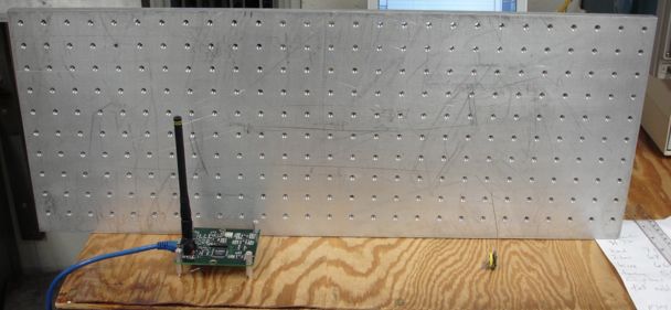
Figure: Reflecting Plate to Observe Destructive Interference. Note the transmitter antenna is vertical in this photograph, but in our reflection experiment, it was lying flat on the table, and perpendicular to the spectrometer antenna.
We turned the transmitter so it lay horizontal and tangential to the spectrometer antenna. We moved the plate around at all angles, ranges, and positions. With the plate far away, the received signal was +22 dBi. With the plate brought close, we were able to increase the received power to +40 dBi, which compares well to the +44 dBi we get with the antenna vertical. But we were also able to decrease the received power down to 0 dBi by holding the plate with one corner resting on the table, and angling up at a compound 45° angle to the antennas.
Increasing the power of our transmitter would not help us overcome reflections. The reflections would become more powerful also. There are four things we can do to reduce the power of reflections with respect to the power of the stright-line transmission.
- Use two receivers instead of one, as we proposed and demonstrated here. We found that the chances of destructive interference occuring at two receiving antenna at the same time are small, and reception from two antenna was robust. We will not be able to produce a dual receiver for Stage Three of development, but if necessary, we can produce one for Stage Four.
- Keep large reflecting bodies away from the transmitter and receiver. This includes our own bodies. But this will be difficult in modern laboratories, where animal cages may be on shelves with iron girders in the walls.
- Transmit power equally in all directions. Our quarter-wave antenna transmits more powerfully perpendicular to its length. If we transmitted equally in all directions, we would never radiate along a reflective path with more power than we do along the straight-line path.
- Receive power equally with vertical and horizontal polarization. Our dipole antenna, being vertical, is far more sensitive to radiation with vertical polarization.
We transmit a thousand times as much power as we need to overcome interference at ranges up to 30 cm. But no matter how much power we transmit, the assymmetry in our transmitting and receiving antennas makes us vulnerable to reflections. In the section below, we show how we can sacrifice radiation efficiency for symmetry, and so make our reception less vulnerable to reflections.
Omnidirectional Antennas
In our laboratory, we receive 30 dBi from an A3009R at 100 cm (see above). Rat bodies and cage walls will attenuate our signal by no more than 6 dB (see above). At one meter, we expect to receive at least 24 dBi. We can receive a signal reliably so long as it is at least 12 dBi. So it looks as if we have 14 dB of extra power. And yet we still find our transmission to be unreliable at ranges as short as 30 cm.
All the above measurements we performed with a vertical dipole antenna on our receiver (either the spectrometer or the data receiver) and a vertical quarter-wave antenna on our transmitter. Both these antennas are omnidirectional in the horizontal plane. We put the receiver on the table with its antenna vertical and it is sensitive to vertically-polarized radio waves anywhere on the table. The transmitting antenna, when it is vertical, transmits powerfully in a horizontal plane, and with vertical polarization. Under these conditions, our reception is reliable to at least 200 cm.
Our reception becomes unreliable when we rotate the transmitter, and the reception is unreliable not because we do not receive enough power at the receiver. It becomes unreliable because of reflections. The straight-line signal to the receiver is powerful enough, but it can be cancelled by destructive interference with an equally-powerful reflected signal.
At first glance, we might doubt that a reflection could be as powerful as the straight-line signal. But there are two ways in which a reflection can gain an advantage over the straight-line signal.
First, suppose the transmitter is horizontal. It transmits horizontally-polarized waves. The receiving antenna is insensitive to these, prehaps only 10% as sensitive as it is to vertically-polarized waves. But a suitably-oriented reflector can rotate the polarization of the reflected wave so that it is near-vertical. Although the reflection travels farther, the receiver is more sensitive to the reflected power.
Second, the transmitter with quarter-wave antenna does not transmit uniformly in all directions. In the direction of its length, it may transmit with only 10% the power as it does perpendicular to its length (see How Antennas Work here). Suppose the transmitting antenna is pointing towards the receiver, but parallel to a reflecting surface. The straight-line path is 100 cm and the reflected path is 300 cm. The reflected signal starts off its journey 10 dB (ten times) more powerful than the straight-line signal, but in travelling three times farther, it drops to the same power of the straight-line signal when it arrives, which is just right for destructive interference.
None of this could happen if our receiving antenna were sensitive to radiation of both polarizations, and our transmitting antenna radiated equally in all directions. The reflections could never match the power of the straight-line signal, and so they would never be able to destroy the straight-line signal by interference. We would like to equip our receiver with an omni-polar antenna, and our transmitter with an omni-directional antenna.
Let us begin by rotating a straight dipole transmitting antenna in front of a straight dipole receiving antenna. We arrange our spectrometer and modulating transmitter 50 cm apart, as shown below.
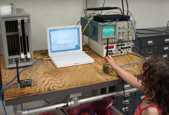
Figure: Dipole-Dipole Transmission Test. Alice holds the modulating transmitter. The spectrometer is on the left.
We drove the modulating transmitter with a 10-kHz square wave to spread its spectrum out through the 900-MHz ISM band. We rotate the antenna about the line between its center and the center of the receiving antenna (that's towards Alice in the picture). We also raise the antenna off the table by a few centimeters in a couple of orientations. Below you see the range of spectra we obtained.
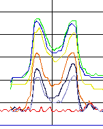
Figure: Dipole-Dipole Reception Power With Orientation. Each vertical division is 10 dB increase in received power. Range is 50 cm. Red (A): background, Green (B) 0° from vertical, Blue (C) 45°, Orange (D) 90°, Black (E) 90° raised off table, Yellow (F) 135° raised off table, Gray (G) 270° flat on table. The raw data is here.
When the antenna is vertical, we receive up to four hundred times (26 dB) more power than when it is horizontal. In theory, a quarter-wave antenna will behave the same as a dipole-antenna. Cleary, we have a problem if we want to implant our quarter-wave antenna in a rat. The rate will rotate.
We previously observed that the length of a quarter-wave antenna has a strong effect upon its power output, but its shape does not. So we replace our modulating transmitter's dipole antenna with the bent quarter-wave antenna shown below.
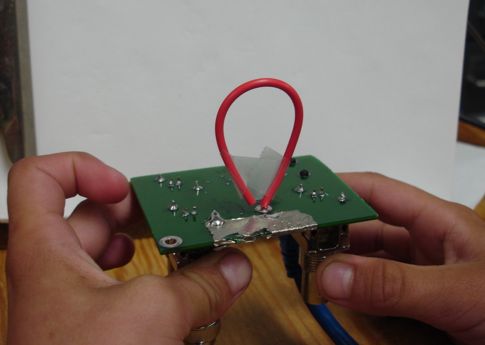
Figure: Bent Quarter-Wave Antenna on Bottom Side of Modulating Transmiter (A3001A). The rubber-insulated wire is 80 mm long. The hands are Haley's.
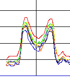
Figure: Dipole-Bent Reception Power With Orientation. Each vertical division is 10 dB increase in received power. Range is 50 cm. Red (A): bend is in direction of receiving antenna and in a vertical plane with ground plane beneath it, Green (B) rotated 45° clockwise, Blue (C) 90° clockwise, Orange (D) bend in horizontal plane, Black (E) plane of bend 45° to horizontal, Yellow (F) as E, but raised by 5 cm off table. The interference background is 6 dB above the blue line. The raw data is here.
Now we see that the highest power received from the bent quarter-wave antenna is +30 dBi, compared to +41 dBi with the straight dipole transmitter. But the lowest received power is +22 dBi compared to +15 dBi with the dipole. Recall that the minimum power required by the receiver is +12 dBi. Furthermore, the power received from the bent antenna changes by only 8 dB as we rotate it, so that the power launched along a reflection path can never be more than 8 dB (six times) greater than that launched along the straight path. With the dipole antenna, however, the difference could be up to 26 dB (four hundred times).
We attached a loop antenna to our Subcutaneous Transmitter (A3009R), number 2.4, and continued our tests with it as our source of RF power. We started with a bare piece of stranded wire for the antenna, fastened into a loop with a 100-kΩ axial resistor. The resistor serves as an insulator with solder leads on either end.
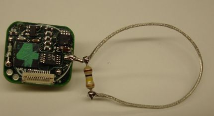
Figure: Bent Quarter-Wave Antenna on Subcutaneous Transmitter (A3009R). Each vertical division is 10 dB increase in received power. The bare wire is 80 mm long. A 100-kΩ resistor holds it in a loop, but acts as an insulator.
We removed the dipole antenna from our RF Spectrometer (A3008) and replaced it with a loop of wire 320 mm in circumference, which is one wavelength of 915 MHz radiation in air. This makes a loop antenna, as we described here.
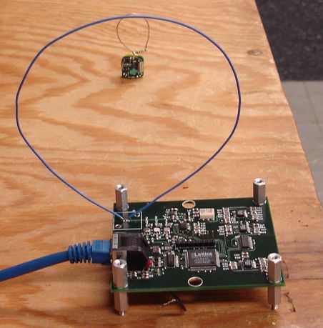
Figure: Full-Wave Loop on Spectrometer and Bent Quarter-Wave on Transmitter. The two are a little over 50 cm apart in this picture, and in our experiments, they were exactly 50 cm apart.
We held the transmitter in a bunch of different orientations at a range of 50 cm. We recorded the spectra below.
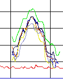
Figure: Loop-Bent Reception Power In Various Orientations. Each vertical division is 10 dB increase in received power. Range is 50 cm. The red (A) trace is the interference background, which we take as 6 dB above the blue line. The raw data is here.
After we recorded the above spectra, we fixed the spectrometer at the peak of the transmission spectrum, and watched the peak power changed in real-time as we continued to rotate the transmitter. The peak power we received was 39 dBi, which is equal to the peak power we received with two aligned dipole antennas. The minimum power we received, in two particular related orientations was 27 dBi.
We now embarked upon a more thorough investigation of the relationship between received power and transmitter orientation. We held the transmitter on the loop axis as shown here. We rotated the transmitter in 30-degree steps in three different ways and recorded the peak power we received.
| Angle (°) | A (dBi) | B (dBi) | C (dBi) | D (dBi) |
|---|
| 0 | 36 | 37 | 38 | 33 |
| 30 | 34 | 34 | 37 | 28 |
| 60 | 30 | 33 | 37 | 28 |
| 90 | 21 | 29 | 37 | 29 |
| 120 | 24 | 27 | 34 | 30 |
| 150 | 30 | 30 | 33 | 33 |
| 180 | 36 | 28 | 32 | 34 |
| 210 | 35 | 33 | 34 | 33 |
| 240 | 30 | 34 | 34 | 27 |
| 270 | 25 | 35 | 35 | 27 |
| 300 | 34 | 37 | 37 | 33 |
| 330 | 35 | 38 | 37 | 34 |
| 360 | 35 | 36 | 38 | 35 |
Table: Power Received from Bent Antenna by Loop Antenna. The transmitter is on the axis of the loop, at range 50 cm. We rotate the transmitter in thirty-degree steps. At 0°, the curvature of the bent antenna is parallel to the loop. A: transmitter beneath its antenna, rotation is away from loop. B: transmitter beside antenna, rotation is away from loop. C: transmitter beneath antenna, rotation is about a vertical axis. D: for comparison, modulating transmitter with dipole antenna vertical at 0° and rotating in plane of loop. The numbers we give are the spectrometer power measurement minus the interference background. The interference background is 6 dB above the blue line in a spectrometer plot, and the blue line is at +20 dB.
The minimum power reception occurs when the bent antenna lies in a horizontal plane and points directly towards or away from the loop (A at 90° and 270°). The received power varies from +21 dBi to +38 dBi across 36 orientations, but is less than +30 dBi for only 6 orientations. Compare this to the dipole-dipole measurements, in which the received power varied from +15 dBi to +41 dBi, with three out of six orientations providing less than +30 dBi.
To measure the sensitivity of our loop antenna to different polarizations of incoming waves, we restored the dipole antenna to our modulating transmitter and measured the sensitivity of our loop antenna along its axis. Our measurements are in column D above. As you can see, our received power varies by 8 dB as we rotate the polarization of the transmitted radio waves. This contrasts with the 26-dB variation we observed with the same rotation and a dipole receiving antenna.
According to web reports like this and this, a loop antenna is sensitive only to polarization in one direction. The symmetry of the loop is broken by its connection to your circuit, and the loop is sensitive only to polarization along the diameter ending at the connection. We should expect our loop to be 20-dB less sensitive to horizontal than vertical polarization. Instead, it is only 8-dB less sensitive. This is because our loop antenna is not resonating well at our operating frequency. We should connect a loop antenna to a 100-Ω load if we want it to resonate well (and even then we will have complications). We connect ours to a 50-Ω load, and this makes the antenna less sensitive to vertical polarization, but more sensitive to horizontal polarization. If we were to connect the loop to a 0-Ω load, its symmetry would no longer be broken, and it would be just as sensitive to horizontal as vertical waves. By connecting the loop to a 50-Ω load instead of a 100-Ω load, we sacrifice sensitivity to one polarization, but gain sensitivity to another, which is exactly what we set out to do.
We end this section with some results we obtained with helical antennas. We did some initial experiments earlier. It seemed to us that the helical antenna could be omni-directional, and when combined with a loop antenna on the receiver, would provide good reception in all orientations. We equipped our A3009R with an ANT-916-JJB-ST from Antenna Factor, as shown below.
Figure: ANT-916-JJB-ST Helical Antenna on A3009R.
We held the transmitter 50 cm in front of the spectrometer with loop antenna and rotated it to get an idea of its radiation pattern. Here are the spectra we obtained.
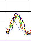
Figure: Power Received from Helical Antenna. Red (A) antenna vertical. Green (B) 30° rotated in plane of receiving loop. Blue (C) 60°. Orange (D) 90°. Black (E) turned from D by 45° towards loop. Yellow (F) pointing straight towards loop. Gray (G) enclosed in one hand, held vertical.
We see that the helical antenna is indeed omni-directional. But it distorts the transmission spectrum when we hold it in one hand. We noticed a similar distortion when we removed the cover of our previous helical antenna. We read here that, "Because a helical has a high Q factor, its bandwidth is very narrow and the spacing of the coils has a
pronounced effect on antenna performance. The antenna is prone to rapid detuning especially in proximity to objects." We conclude that the helix is not suitable for use in animal bodies.
Hand-Held Operation
If our transmitter can operate in open air, and also when clasped firmly in two hands, then we believe it will work inside a rat's body. We tried various lengths of antenna, held them in one hand and then two hands, and measured the power received by our spectrometer. We found that we had to use insulated antenna wire for reliable transmission when clasped in our hand, so we used our red rubber-insulated wire.
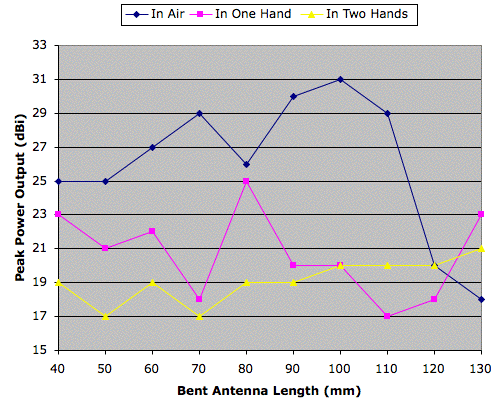
Figure: Power Received by Loop Antenna with Bent Antenna Length. The bent antenna is on the axis of the loop at range 50 cm. We let the transmitter stand on its own, then held it in one hand, then clasped it in two hands. In each case we obtained its power spectrum in the ISM band, and plotted the peak power in the figure.
Our results were erratic, especially with the longer antenna lengths. We suspect that how tightly we gripped the circuit, and its exact location, may have affected our measurements. We don't trust the power measurements shown above to better than ±3 dB.
Despite the inaccuracy of the measurements, it's clear that the bent antenna resonates when it is 110 mm long, not 80 mm. It's not clear, however, that resonance is going to help us. Resonance can cause the antenna to be less omnidirectional. We performed most of our radiation pattern tests on a bent 80-mm antenna. We are not sure if clasping in one hand or two is a good approximation of implanting in a rat, but we guess it's one hand. In that case, we get the most power with an 80-mm bent antenna.
Given the limited space inside a rat, we asked ourselves if we should drop to a 60-mm bent loop for the next batch of four transmitters we ship to London. In the end, we figured that if the antennas are too long, our customer will complain, and we can shorten them for the final version. For now, we will ship transmitters with bent 80-mm antennas.
Operating Range
We replaced the dipole antenna on our Data Receiver (A3010) and recorded the artificial square wave transmitted by our Subcutaneous Transmitter (A3004R) with an 80-mm, insulated, bent quarter-wave antenna, as shown here.
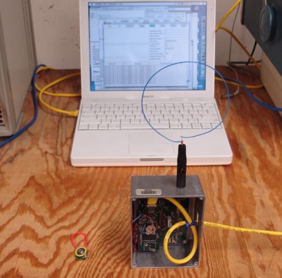
Figure: Apparatus for Estimating Operating Range. The Data Receiver (A3010) has a loop antenna. The Subcutaneous Transmitter (A3009R) has an insulated, bent, quarter-wave antenna.
You can see in the picture that we have the cover of our Data Receiver (A3010) removed. That's because this particular A3010 does not work well when it's cover is on. We have not had time to figure out why it does not work with the cover on, but we made sure not to ship this one to London.
We held the A3009R on our hand, enclosed completely by our fingers so that no part of it was visible. We moved the transmitter around around in front of the A3010's loop antenna, rotating it randomly, looking for reception dead spots. Within 60° of the loop axis, and at ranges less than 1 m from the loop, our reception was reliable regardless of orientation, or bringing another fist near to the transmitter. We sometimes observed the recorder to miss a few samples out of a hundred, but we could not hold the transmitter in a position where such loss was sustained. Reception is less reliable off to the side of the loop, because it starts to look like a quarter-wave antenna from the side, and is sensitive only to vertically-polarized waves.
Our laboratory is full of metal objects and cabinets, but we find that our bent quarter-wave antenna and full-wave loop antenna almost eliminate multi-path interference for ranges up to 1 m within 60° of the loop axis.
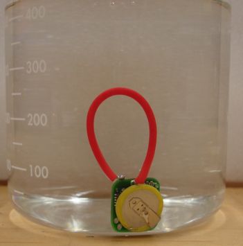
Figure: Coated Transmitter in a Beaker.
We coated transmitter 2.4 twice with silicone, as we describe here. We dropped the transmitter in a beaker of water, and found that it transmitted well enough for reliable reception up to 50 cm within 60° of the loop axis.
We describe the A3009A analog inputs in detail in the A3009 manual, with many attractive pictures of the Recorder output. The analog input impedance is 10 MΩ, its dynamic range is +23 mV down to -50 mV. The stochastic noise on the input, with a 10-MΩ source impedance, is 20 μV. This 20 μV is greater than the expected 10 μV thermal noise, and we believe is due to digital signals coupling to the inputs during the burst transmissions.

Figure: Designed and Measured Frequency Response of Analog Input.
The analog input provides a single-pole high-pass filter with cut-off frequency roughly 0.1 Hz, and a three-pole low-pass filter with cut-off frequency 160 Hz. As you can see from the graph above, the low-pass filter performs as we had hoped.
Peer-to-Peer Interference
When two transmitters start transmitting at the same time, we say that each is suffering from peer-to-peer interference. Below is the recorder output when two A3009R transmitters, which do not have random displacement of their transmission instants, begin transmitting at the same instant for several seconds.
0 278 1.352 0.004 2 1111 0.844 0.094 3 1111 1.219 0.094 -1 1
0 430 1.368 0.006 2 808 0.844 0.094 3 1263 1.218 0.094 -1 0
0 624 1.392 0.008 3 1811 1.221 0.103 -1 66
0 366 1.415 0.005 2 717 0.844 0.094 3 1417 1.219 0.094 -1 1
0 278 1.430 0.004 2 1111 0.843 0.094 3 1112 1.218 0.094 -1 0
0 278 1.442 0.004 2 1111 0.844 0.094 3 1110 1.219 0.094 -1 2
Table:Recorder Results During Collision. The columns are: transitter channel number, number of messages received, average voltage, an rms voltage, for however many channels the recorder hears.
In the table above, the recorder hears channels zero, which is the time stamp channel, without interruption. It gets one time stamp every 7.8 ms. Channel 2 is one transmitter at range 1 m, and channel 3 is another transmitter at range 20 cm. Channel -1 is the corrupted-message channel. We start off with reliable reception from each transmitter, then we see one acquisition in which the nearer transmitter dominates the farther transmitter completely. The two are transmitting at the same time.
The A3009A overcomes peer-to-peer interference by displacing its transmission moment by a number of 32.768 kHz clock cycles equal to the lower four bits of its 16-bit ADC data. Because the lower four bits are dominated by noise on the ADC input, they are random. The transmission itself takes 8 μs. If two transmitter clocks are synchronous, the chance of them both transmitting on the same clock edge is only one in sixteen. This means we will lose no more than one in sixteen samples to peer-to-peer interference.
Transmitters seem to come into synchronization for several seconds at a time once ever ten or fifteen minutes. The chances of three transmitters being synchronous at the same time are small enough to ignore, and even if they were, we would not lose all our information, because of the random transmission displacement.
With a dozen transmitters sharing a single receiver, we can assume that collisions between transmitter occur at random. Each transmitter is active for 8 μs every 2 ms, which is 0.4% of the time. To the first approximation, it will collide with another transmitter for only 4 transmissions out of each thousand. Any pair of transmitters has the same collision frequency. If we have a dozen transmitters, we have sixty-six pairs, so we lose twenty-five percent of transmissions. If we can reject corrupted transmissions with certainty, we will be able to operate perfectly well with 75% of the data. But rejecting corrupted samples will have to be done in software, and remains a question to be answered in Stage Four of development.
Battery Life
See the Subcutaneous Transmitter (A3001) manual for a detailed discussion of transmitter current consumption, and how over-heating the logic chips during assembly dramatically increased the current consumption of our first batch of transmitters.
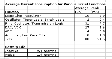
Figure: Current Consumption of Circuit Parts, and Battery Life
If we assume the battery capacity is 120 mA-hr, as advertised in its data sheet, then the A3009's operating life is 2 months, and its shelf life is 9 months.

Figure Battery Voltage During Transmission. The plot begins when the transmitter turns on with a fresh battery, and ends when transmission begins to fail. Transmitter's active current consumption was 94 μA.
We ran one transmitter until it exhausted a fresh battery, with the result shown above. See here for details.
Temperature
The MAX2624's output frequency for fixed input voltage drifts by −0.2 MHz/°C. We calibrate our A3009 to transmit at 915±8 MHz at 20°C. Its modulation spectrum is 20 MHz wide, as shown here. The spectrum can shift 5 MHz in either direction before significant portions of it are rejected by our A3005C's ISM-band SAW filter. This gives us an operating temperature range of -5°C to +45°C, which is ample for use in laboratories and animals.
Assembly
The A3009 uses P0603 resistors and capacitors instead of P0402. The new parts are larger and easier to solder. Our chief problem during assembly is applying the logic chip. Our heat-gun method, where we simply heat the chip on the board until its solder balls melt, damaged the logic chips on our first six A3009s, so that their current consumption was erratic and greatly increased, as we describe here. We made another batch of ten more carefully. Of these, eight worked. One had its logic chip on the wrong way around. Another we suspect is not soldered properly. Of these eight, all but one is behaving well two months later. The one that does not behave well showed a 90-μA jump in its inactive current some time during a month of inactivity without power. Other than that, it works fine.
We have a new toaster oven, which we will try to use in Stage Four of development to make a batch of twenty transmitters. The toaster-oven method is described here, and a hot skillet method is described here as well as the toaster-oven method. With a temperature sensor in the oven, we are confident that we can re-flow the solder balls without over-heating the package.
For calibration of the transmitter's frequencies, see here. For a discussion of the silicone coating, see here. For a picture of teflon-coated silver wire soldered to the transmitter, see here.
Deliveries
We delivered an RF Spectrometer (A3008) to ION in March 2006.
Transmitters 1.2 and 1.3, which we shipped to ION in April 2006, were A3009Rs programmed to transmit at 915±8 MHz (see parameters). They did not have C11 installed, so they produced one quarter power. Matthew reports that they were reliable up to 3 m in his laboratory for a while, but then drained their batteries. We found the same problem with other in our first batch of six transmitters. As we describe here, we determined that over-heating the logic chips during assembly causes their current consumption to jump around during operation. We made another batch of ten transmitters, this time being more careful not to over-heat the logic chips during assembly.
We shipped a Data Receiver (A3010) to ION in April 2006 along with the two transmitters. We equipped the receiver with a commercial dipole antenna.
Transmitters 2.2 and 2.7, which we shipped to ION in May 2006, were A3009Rs programmed to transmit at 915±12 MHz (see parameters). These transmitters did not have C11 installed either, and so produced one quarter power. Along with the other six working transmitters from our second batch, these two show steady current consumption. We shipped them to ION in May 2006, were programmed to transmit at These will give a strong signal at 20°C, but they are unlikely to work well in a live rat, because their power spectra are too wide, like the blue trace shown here.
We shipped a second Data Receiver (A3010) to ION in May 2006 along with the second pair of transmitters. We equipped the receiver with a commercial dipole antenna.
Conclusion
With our bent quarter-wave transmitting antenna and full-wave loop receiving antenna, we eliminate reception dead spots caused by reflections for ranges up to 100 cm, provided we stay within 60° of the loop's axis. With the same combination of antennas separated by 50 cm, our signal is a almost always a thousand times more powerful than the interference in our basement laboratory. The animal laboratory in Lodon has roughly ten times the interference power in the 900-MHz ISM band, so we expect our transmitters to dominate interference there by a factor of a hundred at a range of 50 cm. We find that a factor of sixteen is adequate for proper reception or our 5-MHz data burst. The transmitter should operate reliably up to 100 cm in London also.
In the long run, perhaps we can integrate the transmitter's loop antenna onto its circuit board, as described here and here. For now, we use a bent quarter-wave antenna.
Our battery life agrees with our predictions: 1.8 months for a transmitter with higher than average quiescent current. Our target battery life was 2 months.